Why We Need Alternative Stochastics

Anyone who teaches probability and statistics at school is familiar with two fundamental issues: the empirical law of large numbers and the inference from a sample to the population.
In the established school approach to probability, students are told that, according to the empirical law of large numbers, the relative frequency of an event must approach the probability of that event when the random experiment is repeated many times.
Yet, as can be read in any introductory textbook on probability theory, this is not true — and students notice this. They realise that if you cannot get 100 heads in 100 coin tosses, or if you cannot draw the red ball 100 times from a box containing one red and four blue balls, then these would simply not be random experiments.
This leads directly to the second issue: if the proportion of red balls in a sample does not have to correspond to the proportion of red balls in the population, we cannot legitimately draw conclusions from the sample to the population. And again, students notice this.

Alternative stochastics provides very clear solutions for both problems:
Probability theory: Probabilities are assigned to the possible relative frequencies that can be drawn from a given population.
Statistics: Probabilities are assigned to the possible populations from which a certain relative frequency can be drawn.
With these principles, there is no longer any need to speculate whether the relative frequency must, could, or should approach the probability (perhaps after a very large number of trials). Nor is there any need to use a procedure — which, in any case, one cannot reasonably „sell“ — to exclude possible populations for a given sample simply because they fail to satisfy arbitrarily imposed conditions.

Directly Inferring Statistics – A wholesome way to understand the big picture

Doing statistics is often like this: We survey 100 people and ask whether they like chocolate — then we transfer the result to the entire population.

Remember back in school: Did you ever understand why statistics are supposed to work at all — giving you information not only about the 100 people you surveyed, but also about everyone you didn’t survey?

With directly inferring statistics, we now have a way to do statistics in a mathematically correct and intuitive way from day one in stochastics class because from the very start, all we need is to count blue and red balls in boxes.

Directly inferring statistics is so easy to understand because it replicates what we humans do every day anyway: We assign probabilities to possible populations.

Directly inferring statistics is easy to teach, because the principle remains exactly the same from start to finish: divide the number of certain samples by the number of all samples.

Directly Inferring Statistics – The Method.pdf

Directly Inferring Statistics – Problems, Grades 6 – 8.pdf

Directly Inferring Statistics – Problems, Grades 9 – 10.pdf

Directly Inferring Statistics – Problems, Grades 11 – 12.pdf

A Simple Example

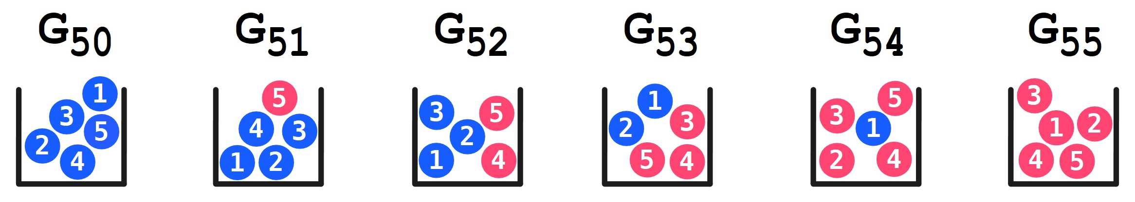
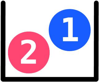
Let’s dive into an example which is as simple as possible, but not simpler. Imagine we have a Box with 5 balls which are either blue or red. We draw a random sample with replacement of size 3. Suppose we have drawn one blue ball and two red balls. How can we now infer from the sample to the population? How many balls in the box are red?

There are 6 possible proportions of red balls in boxes with 5 balls. (For the sake of arbitrariness, we will focus on the red balls here.)

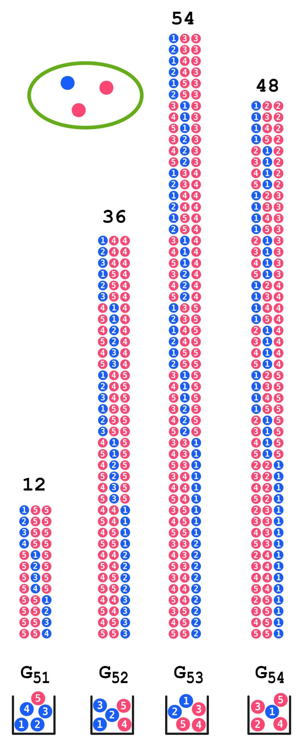
We can now draw which possible samples of size 3 with 2 red balls can be drawn from each of the boxes, omitting \(G_{50}\) and \(G_{55}\) from the diagram. From \(G_{51}\), 12 samples with exactly 2 red balls can be drawn, from \(G_{52}\) there are 36, from \(G_{53}\) there are 54, and from \(G_{54}\), 48 samples with exactly 2 red balls can be drawn. A sum of 150 samples can be drawn from all boxes.

To determine the probability of drawing the current sample from a given box, we divide the number of possible samples (of size 3 with exactly 2 red balls) from a given box by the sum of all samples (of size 3 with exactly 2 red balls) from all boxes.

The probabilities are:

\(\mathbf{P}(G_{51})=\frac{12}{150}=\frac{2}{25}=0.08\)

\(\mathbf{P}(G_{52})=\frac{36}{150}=\frac{6}{25}=0.24\)

\(\mathbf{P}(G_{53})=\frac{54}{150}=\frac{9}{25}=0.36\)

\(\mathbf{P}(G_{51})=\frac{48}{150}=\frac{8}{25}=0.32\)

Returning to the question posed at the beginning: What do we know about the balls we did not draw? Well, although we know nothing about the individual balls, we can specify the probabilities with which the present sample can be drawn from which population.

As expected, the populations with the highest probabilities are those that are most similar to the sample in terms of the proportion of red balls. Population \(G_{53}\), with a population proportion of \(\frac{3}{5}\) red balls, has the highest probability \(\mathbf{P}(G_{53})= 0.36\).

This phenomenon, which is ultimately based on combinatorics, runs through the entire field of statistics and should therefore be formulated as simply as possible in the main theorem of statistics:

Most samples come from similar populations.

There are surprisingly many situations in which such simple tasks can be applied:
Let’s imagine we are students and new to a school. We have been to the cafeteria three times, and once it was empty and twice it was full. What is our prediction for the future?
Since we only have a small sample size, we divide our expectations roughly: Either the cafeteria is

• rarely full (20% full) or
• occasionally full (40% full) or
• often full (60% full) or
• mostly full (80% full).

We can simulate this situation with our boxes with 5 balls. So we have only 4 boxes to choose from. What we then expect the most for our next visit of the cafeteria is that the cafeteria ist often full, we do not expect that it is rarely full.

The Empirical Law of Large Numbers

Suppose we have a box containing one blue ball and one red ball. We randomly draw a ball, record its color, and then put the ball back. We repeat this process, drawing a ball each time, and continue in this way. If we carry out this procedure \( 100\) times, it is quite likely that we will draw approximately \(50 \) blue balls and approximately \(50 \) red balls. This „fact“ is the core statement of the empirical law of large numbers. But why is this the case? Certainly not because the „laws of chance“ demand it—as is sometimes grandiosely claimed. (And even if that were true, the question of „why?“ would still remain unanswered.) The shortest possible answer is: Because there are far more possible sequences with approximately \(50 \) blue balls than there are sequences with other distributions.

However, we do not need to carry out the random experiment 100 times to recognise the system. As can be seen in the figure, 8 attempts are enough to realise that most of the possible sequences of blue and red balls contain around 50% red balls.

In the following PDF, the situation is explained in detail. It precisely defines what is meant by „far more possible sequences“ and also shows how the empirical law of large numbers can be understood using the Galton board. Furthermore, it demonstrates how, even without knowledge of combinatorics, the numbers of possibilities can be calculated for the first few trials using (extended) Pascal’s triangles.

The unique method of explaining the empirical law of large numbers presented in the PDF has the enormous advantage that the regularities can be recognized intuitively after only the first few trials. Therefore, it is possible to omit the usual (and often confusing) note that the empirical law of large numbers applies only to very, very many trials.

The claim that the relative frequency of an event must approach the probability of that event when a random experiment is repeated „many“ times is frequently (and incorrectly) cited as the central statement of the empirical law of large numbers. There are many formulations of this, some more incorrect than others. A completely false formulation can be found (at least, it could be found there), for example, on the pages of the MUED e. V. association (for members):

„This famous law of large numbers states that, in many independent repetitions of a random experiment—whether coin tosses, dice rolls, lottery draws, card games, or anything else—the relative frequency and the probability of an event must always come closer together: The more we toss a fair coin, the closer the proportion of ‚heads‘ approaches its probability of one-half; the more we roll dice, the closer the proportion of sixes approaches the probability of rolling a six; and the more we play the lottery, the closer the relative frequency of drawing the number 13 approaches the probability of 13. There is no disputing this law; in a sense, this law is the crowning achievement of all probability theory.“

Why This Is So Important:

To put it very briefly: If this law were correct in this formulation, there would not exist a single (repeatable) random experiment.

An example: Suppose we toss a coin randomly, so that the outcomes H (heads) and T (tails) are possible. Each outcome is supposed to have a probability of 0.5. Further, suppose we toss the coin 50 times and obtain T every single time. Then the relative frequency of T after the first trial was 1, after the second trial it was still 1, and the same after the third, fourth, and so on. In these first 50 trials, the relative frequency of T did not approach the probability of T at all.

It is often argued that the relative frequency and probability „approach each other in the long run“ or „after very many trials.“ But what is that supposed to mean? Does the coin, if it showed T too often in the first 50 trials, have to show H more frequently until the 100th trial to restore the balance? Or must the relative frequency only approach the probability by the 1000th trial?

No matter how we look at it: If relative frequency and probability must approach each other, the outcome of a coin toss could no longer depend on chance at some point, but would have to follow what the coin showed in the previous trials. In that case, the coin toss would no longer be a random experiment. One may debate what exactly randomness is, but it is certainly part of a random experiment like a coin toss that there is no law dictating what the coin must show.

The situation becomes even worse when, in an introductory course on probability, it is claimed that the probability of an event is the number toward which the relative frequency of the event “tends” if the random experiment is repeated sufficiently often. Apart from the fact that students have no clear understanding of what “tends” or “sufficiently often” means, they also cannot reconcile such a “definition” with their conception of randomness. This approach leads to the absurd idea that someone must tell the coin what to do, or that the coin has a memory and actively seeks to balance relative frequency and probability. As a result, the fundamental concepts of probability theory—namely, randomness and probability—become so contradictory that a student’s understanding of this area of mathematics is effectively impossible.

Unnecessary Statistics

One can read in any book on the introduction to probability theory that the relative frequency of an event does not have to approach the probability of that event, even after an arbitrarily large number of trials. All statistical methods that infer probability from relative frequency would be unnecessary if relative frequency were required to approach probability. The concepts of “convergence in probability” and the weak law of large numbers exist precisely because the relative frequency of an event does not analytically converge to the probability of the event. Why, nevertheless, incorrect mathematics is still taught in German schools is, for me personally, incomprehensible.

The empirical law of large numbers is not by Bernoulli

It is often claimed that Jakob Bernoulli (1654–1705) was the first to formulate the empirical law of large numbers. However, that is not correct—at least not if one considers the common formulations of this law. Bernoulli did not write that the relative frequencies of an event A settle, for a sufficiently large number nnn of repetitions, at the probability of A. Nor did he write that the relative frequencies of an event A stabilize, as the number of trials increases, at the probability of A. And he also did not write that the relative frequencies of A must approach the probability of A as the number of trials increases.

This is, what Bernoulli actually wrote:

„Main Theorem: Finally, the theorem follows upon which all that has been said is based, but whose proof now is given solely by the application of the lemmas stated above. In order that I may avoid being tedious, I will call those cases in which a certain event can happen successful or fertile cases; and those cases sterile in which the same event cannot happen. Also, I will call those trials successful or fertile in which any of the fertile cases is perceived; and those trials unsuccessful or sterile in which any of the sterile cases is observed. Therefore, let the number of fertile cases to the number of sterile cases be exactly or approximately in the ratio \(r\) to \(s\) and hence the ratio of fertile cases to all the cases will be \(\frac{r}{r+s}\) or \(\frac{r}{t}\), which is within the limits \(\frac{r+1}{t}\) and \(\frac{r-1}{t}\). It must be shown that so
many trials can be run such that it will be more probable than any given times (e.g., \(c\) times) that the number of fertile observations will fall within these limits rather than outside these limits — i.e., it will be \(c\) times more likely than not that the number of fertile observations to the number of all the observations will be in a ratio neither greater than \(\frac{r+1}{t}\) nor less than \(\frac{r-1}{t}\).“ (Bernoulli, James 1713, Ars conjectandi, translated by Bing Sung, 1966)

German translation (slightly different):

„Satz: Es möge sich die Zahl der günstigen Fälle zu der Zahl der ungünstigen Fälle genau oder näherungsweise wie , also zu der Zahl aller Fälle wie \( \frac{r}{r+s}=\frac{r}{t} \) – wenn \( r+s=t \) gesetzt wird – verhalten, welches letztere Verhältniss zwischen den Grenzen \( \frac{r+l}{t} \) und \( \frac{r-l}{t} \) enthalten ist. Nun können, wie zu beweisen ist, soviele Beobachtungen gemacht werden, dass es beliebig oft (z. B. c-mal) wahrscheinlicher wird, dass das Verhältniss der günstigen zu allen angestellten Beobachtungen innerhalb dieser Grenzen liegt als ausserhalb derselben, also weder grösser als \( \frac{r+l}{t} \) , noch kleiner als \( \frac{r-l}{t} \) ist.“ (Bernoulli 1713, S. 104), in der Ausgabe: Wahrscheinlichkeitsrechnung (Ars conjectandi), Dritter und vierter Theil, übersetzt von R. Haussner, Leipzig, Verlag von Wilhom Engelmann, 1899)

What Bernoulli actually wrote is, in fact, correct and comes very close to the weak law of large numbers.

Computationally impossible

There are infinitely many possible situations in which the relative frequency of an event does not approach the probability of that event but instead diverges from it.

An example: Suppose we toss a coin randomly, so that we can obtain the outcomes T (Tails) and H (Heads). Both outcomes are assumed to have a probability of \(0.5\). Now, suppose we have tossed the coin \(100\) times and obtained \(50\) T and \(50\) H. Then the relative frequency of T is \(0.5\). If we toss the coin once more, we will either get T — in which case the relative frequency of T becomes \(0.\overline{5049}\) — or we will get H — in which case the relative frequency of T becomes \(0.\overline{4851}\). In both cases, the relative frequency of T moves away again from the probability of T. If, after obtaining T on the 101st trial, we continue to obtain T on subsequent trials, the relative frequencies of T will be as follows:

\(\approx 0.5098\), \(\approx 0.5146\), \(\approx 0.5192\), \(\approx 0.5283\), usw.

Thus, the relative frequency of T moves farther and farther away from the probability of T, which contradicts the so-called Law of Large Numbers.

Unusual Sequences

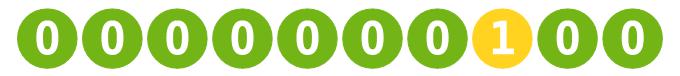
The empirical Law of Large Numbers is often justified by saying that unusual outcomes may occur, but they are so unlikely that they practically never happen. For example, in 30 coin tosses, the outcome HHHHHHHHHHHHHHHHHHHHHHHHHHHHHH is said to be very unusual and also unlikely, while the outcome HTTHTHHHTHTTHTTTHTTHTHHTTTTHT is considered much more normal and therefore more likely.

This is not only wrong because both outcomes have exactly the same probability, but also because we humans imagine the unusualness of certain outcomes into the outcomes themselves. In other words, the coin “knows” nothing about unusual results. Let’s look at an example:

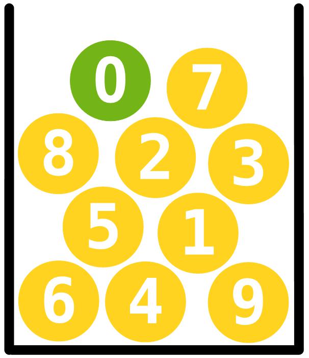
Let’s assume we have ten balls labeled with the digits from 0 to 9. The ball labeled 0 is green, and all the others are yellow. We draw ten times at random, with replacement and with order.

If we only pay attention to the colors, we would probably not consider the result

unusual. But if, upon examining the digits, we discover the following sequence

the sample would probably be regarded as unusual.

Let’s assume we have ten balls labeled with the digits from 0 to 9. The ball labeled 0 is green, and all the others are yellow. We draw ten times at random, with replacement and with order.

If we only pay attention to the colors, we would probably not consider the result

unusual. But if, upon examining the digits, we discover the following sequence

the sample would probably be regarded as unusual.

However, we can set entirely different standards if we wish: we might decide that a sample is to be considered unusual if its sequence of digits appears in the first decimal places of π. The sample

is ordinary, because it does not occur even within the first \(200\) million decimal places of π. The sample

is unusual, because it occurs at position 3,794,572. The sample

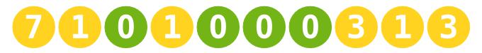
even appears at position 851 and is therefore extremely unusual.

Whether unusual or not, the probability of each sample is exactly the same, namely \[\frac{1}{10\,000\,000\,000}\]

What actually holds true

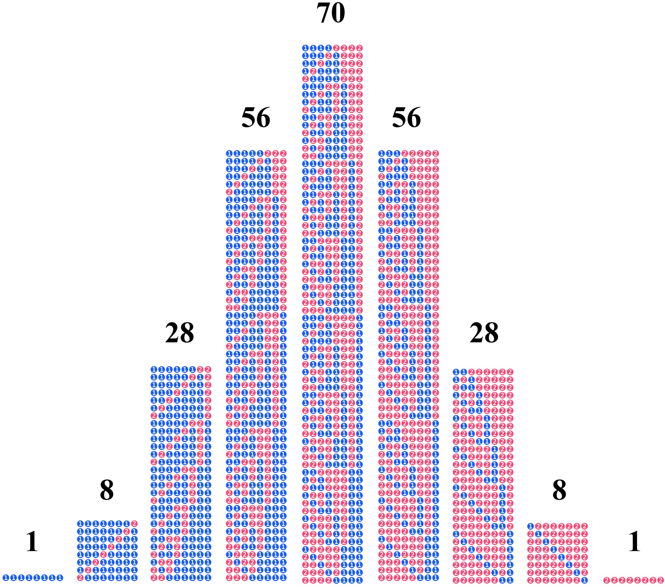
Let’s look at an example: We randomly draw one ball from a box containing two balls. One ball is blue, and the other is red. We draw several times, with replacement and with order.

We will now focus on the numbers of red balls. In the following tables, these numbers are listed depending on the number of trials performed. For example, when drawing eight times, there are 56 outcomes with exactly 3 red balls.

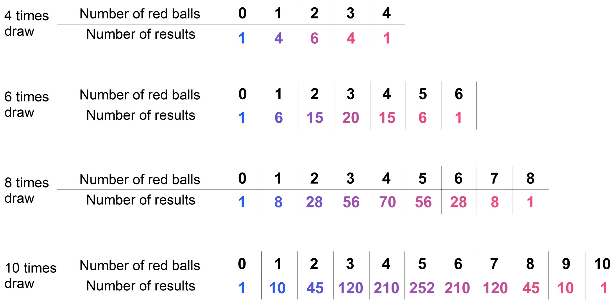
These numbers are represented to scale in the following bar charts. As we can see, with an increasing number of trials, the numbers of outcomes in the middle grow much faster than those at the edges. The more often we perform the experiment, the greater the differences become between the middle and the edges.

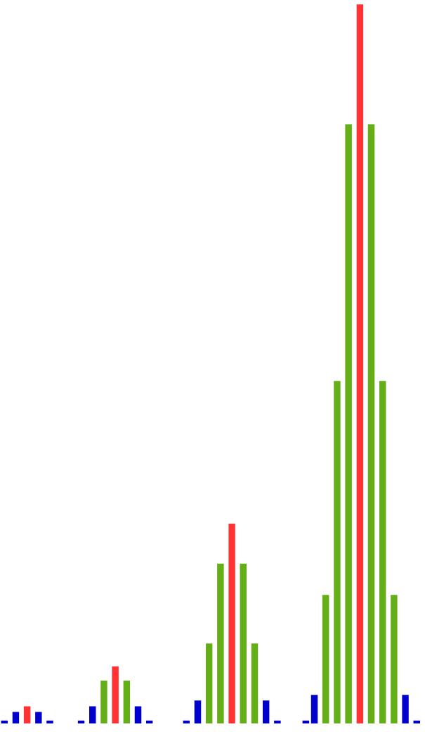
That means: There are simply far more outcomes with approximately 50% red balls than there are outcomes with much fewer or much more red balls. And the proportion of outcomes near the center becomes larger and larger as the number of trials increases.

We can observe this phenomenon also with other proportions of red balls in the population: If two-thirds of the balls in the population are red, we see a clustering of outcomes with about two-thirds red balls.

What we see here can be summarized—somewhat simplified, but not incorrectly—by the following statement: The relative frequencies of red balls are, in most outcomes, similar to the probability of drawing a red ball.

In statistical terms, this sounds like this: Most samples are similar to the population.

So if we flip a coin 100 times and get about 50 H, this is not because the relative frequency stabilizes, or because the coin strives for a balance between H and T, or because some dark force influences the fall of the coin — but simply because there are far, far more outcomes that contain about 50 H than outcomes that contain much fewer or much more H.

The Weak Law of Large Numbers

The weak law of large numbers holds true. Applied to the case above, this law, stated in simplified form, means that the relative frequency does not have to approach the probability, but rather that the probability of it being close increases.

More precisely: We can ask how large the probability is that the relative frequency of red lies within a certain interval around the probability of red. Since the probability of red is 0.5, we can, for example, set the interval to (0.4, 0.6). The probability that the relative frequency of red falls within this interval becomes increasingly larger as the number of trials increases.

If a red ball was drawn on the first trial, the probability of drawing a red ball on the second trial is just as large as on the first trial, namely \(0.5\). The same applies to other numbers of trials: for example, if after 99 trials 99 red balls have been drawn, the probability of drawing a red ball on the 100th trial is still \(0.5\). And this also holds if 99 blue balls were drawn before, or if any other combination of blue and red balls was obtained.

That means: the probability of drawing 100 red balls is just as large as the probability of drawing any other combination of blue and red balls. Therefore, after 100 trials, the relative frequency of red balls can be equal to 1. In that case, it is as far away as possible from the probability of drawing a red ball and not close to \(0.5\). The same reasoning applies for 1,000, for 10,000, and for any other number of trials. Thus, there is no number of trials — no matter how large — for which it must be true that the relative frequency of red balls lies close to \(0.5\). Therefore, as the number of trials increases, the relative frequency of red balls does not have to approach the probability of drawing a red ball.

Widely Known Problems