
… are wanted here.
Everyone learns differently, and everyone has a unique understanding of mathematics. Therefore, each person needs an explanation of a mathematical concept that is tailored to them. For everyone, there is one explanation that stands out as the best—the best explanation in the world.
Explanations as a Starting Point
On this page you will find a number of explanations—especially ones that you won’t normally encounter in schoolbooks and that go much deeper than what is common among YouTubers or TikTokers. These explanations invite a critical engagement with the material currently taught in schools. To some, this may seem unusual, since mathematics is often regarded as a rigid set of rules. But it is not. There is plenty of “evidence” for that right here.
The explanations presented here are neither the only “correct” ones nor are they complete. Rather, they are meant to serve as a starting point for delving more deeply into the topics. Engaging with mathematics in depth is an exciting journey into your own inner world of structures, logic, and abstraction. May the following ideas help guide you along that path.
Unique Explanations
Almost everyone has the desire to be unique and to be valued for that uniqueness. In mathematics, individuality begins with the fact that each person develops their own understanding of mathematical objects.
Take fractions as an example: they can be seen as parts of a whole, as two-dimensional numbers, as results of division, as outcomes of distribution, as mathematical operators, as points on the number line, as ratios, or as shares. Fractions can be represented with fraction strips, pie charts, or subdivisions of a time span. They can be experienced by sensing different weights, by perceiving different levels of brightness, or by hearing different volumes. All pitches, for instance, arise from different subdivisions of time, and a sound can be described as a tone with differently weighted overtones—again expressible as fractions.
Every student who encounters the topic of fractions will, out of these many possibilities, form their own personal picture of what fractions are. It cannot be otherwise. Realizing this individuality can be a strong motivation to want to learn more about mathematics.
New Mathematics
For some of the explanations on this page, you will also find further questions—questions without standard solutions. Engaging with these questions can quickly lead to new mathematics. Many people assume that students cannot discover anything new in mathematics, but the opposite is true: as soon as you step beyond the usual school exercises and phrase the questions even slightly differently from the way they appear in textbooks, you may arrive at mathematical ideas that have never been published before.
The likelihood of inventing—or discovering—new mathematics in this way is actually quite high. And the joy of making your own contribution to the “history of mathematics” is priceless.
Get Involved
If you know of an explanation that you find helpful but that isn’t yet on this page, send it to me and I will publish it here (as long as it is mathematically correct).
If you are looking for an explanation that isn’t included, feel free to write to me at martinwabnik@gmail.com. We will find someone who can explain it.
Any constructive feedback is, of course, always welcome!
Arithmetic
The Beginning of Mathematics
Fractions
Expressions and Equations
Associative and Commutative Law
Why a Negative Times a Negative Is Positive
Calculus
Fundamental Theorem of Calculus
Probability and Statistics
Empirical Law of Large Numbers
Why the Relative Frequency Does Not Have to Approach Probability
Miscellaneous
Introductory Teaching Video: Volume of a Plate
The Standard Model of School Mathematics
Surface of a Sphere – Cosmetics and Nanoparticles
Martin Wabnik’s YouTube Channel
This YouTube channel offers over 400 high-quality mathematics videos covering various topics in school mathematics. The focus is on developing a deep understanding of mathematics, not on providing empty, mechanical solution recipes. Every video is built on a clear didactic concept, carefully executed both visually and verbally. Anyone who truly wants to understand mathematics will find here exactly what they have been looking for.
Arithmetic
The Beginning of Mathematics
When people are asked where mathematics begins, the most common answer is:
“One and one is two.”
This is often accompanied by the opinion that this statement is proven, indisputably true, will always remain so, and therefore nothing new can arise in mathematics.
However, all of these opinions are factually incorrect. Since there are approximately 100,000 publications worldwide each year containing new mathematics, it cannot be said that there is nothing new in this field.
The reason this statement is often considered indisputable and proven may be that adults have possibly forgotten how much cognitive effort they had to invest as children to learn counting and arithmetic. Here, a few aspects of addition are presented to show that even the statement “one and one is two” can and must be shaped individually. To practice mathematics seriously, we should understand what our starting point can be. There are several meaningful possibilities for this, but they are not simply given; they must be worked out.
Is 1 Plus 1 Equal to 2 ?
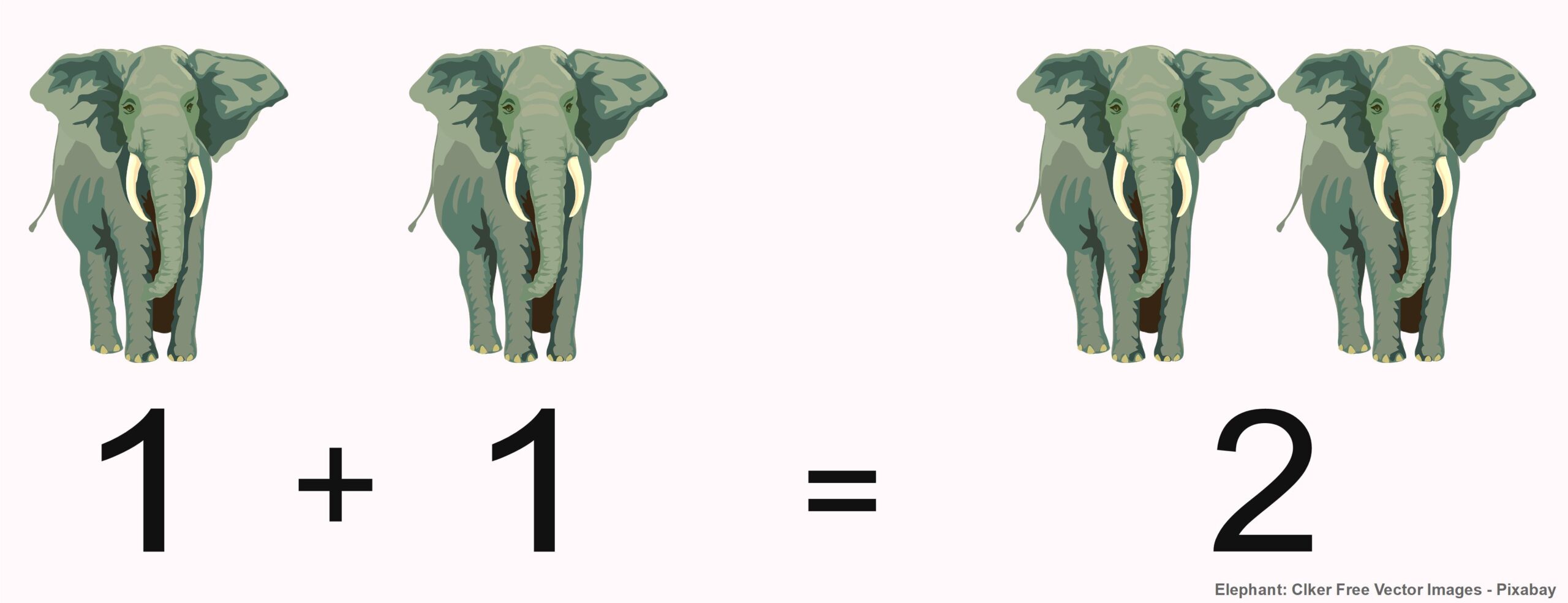
The adjacent image could illustrate the statement: One elephant and another elephant are two elephants. But how do we know that? Most people—at least those who read this sentence—have never counted real elephants in their lives. In school, counting and arithmetic are taught using many different materials, typically with dice, counting tiles, number rods, and perhaps also with apples and pears.
Thus, to recognize an addition in this image, we must be able to come to the somewhat amusing conclusion that elephants are like apples and pears—at least regarding their countability. To seriously maintain this statement, we must be able to distinguish it with our common sense from all sorts of nonsense, which will be demonstrated in the following.
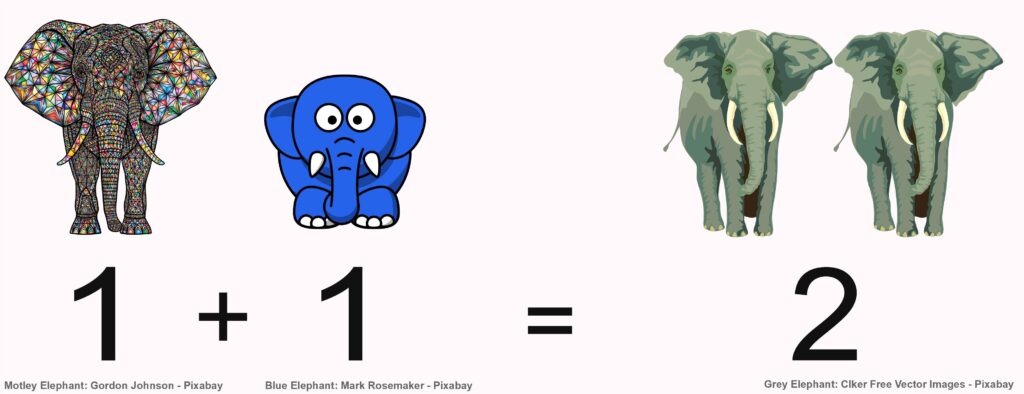
There are no elephants corresponding to the first two illustrations. Can we still add them? A serious question: To what extent must things exist if we want to add them? Can we also add imaginary concepts? We sometimes say, “I just had two thoughts at once.” So, can thoughts be counted? Do they need to occur simultaneously, or is it sufficient if they occur consecutively? We will not be able to definitively resolve these and similar questions. However, they demonstrate that the statement “One plus one is two” cannot be unconditionally true if we cannot even determine to what it is meant to be applied.

What can we apply numbers and calculations to with complete certainty? For example, when baking a cake. If the recipe states that \(2\) eggs are to be added, we add eggs to the batter until we have counted to \(2\). Viewed this way, counting and calculating is a practical mental concept that works perfectly in everyday life. However, this has nothing to do with absolute truth.
- If „adding two eggs“ means to take eggs in our hands and incorporate them into a cake batter, the question arises whether one can add elephants, since it is not so simple to add them to anything—at least, this is more difficult than with eggs.
- If we add \(2\) eggs to a batter, i.e., calculate \(1+2\), we obtain only one batter. In this case, is \(1+2=1\)?
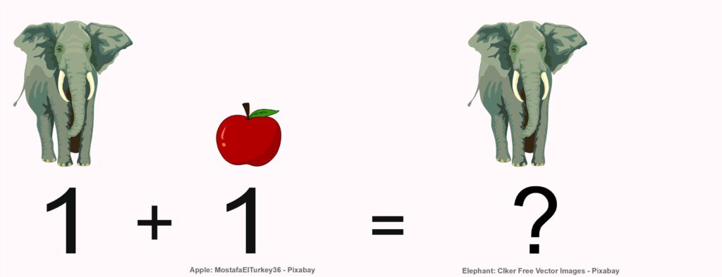
Can we add an elephant and an apple even if the elephant eats the apple?
If one adds an apple to an elephant, one does not end up with \(2\) objects, but only one, because the elephant will likely eat the apple. And even if it does not, what could the \(2\) represent? Two completely unspecified objects? As we can see from these questions, the things we want to add should be sufficiently similar and temporally constant. However, what this similarity should be cannot be defined in general, just as the minimum time span during which things should remain unchanged in order to be addable cannot be generally specified.
We can also understand addition in a completely abstract way as a method that assigns a third number to two given numbers. For example, the numbers \(2\) and \(6\) are assigned the number \(8\), and the numbers \(7\) and \(3\) are assigned the number \(10\). The first assignments can be seen in the table on the right. To obtain further ones, a set of rules — such as the standard algorithm for addition — could be defined, allowing all other numbers to be added as well.
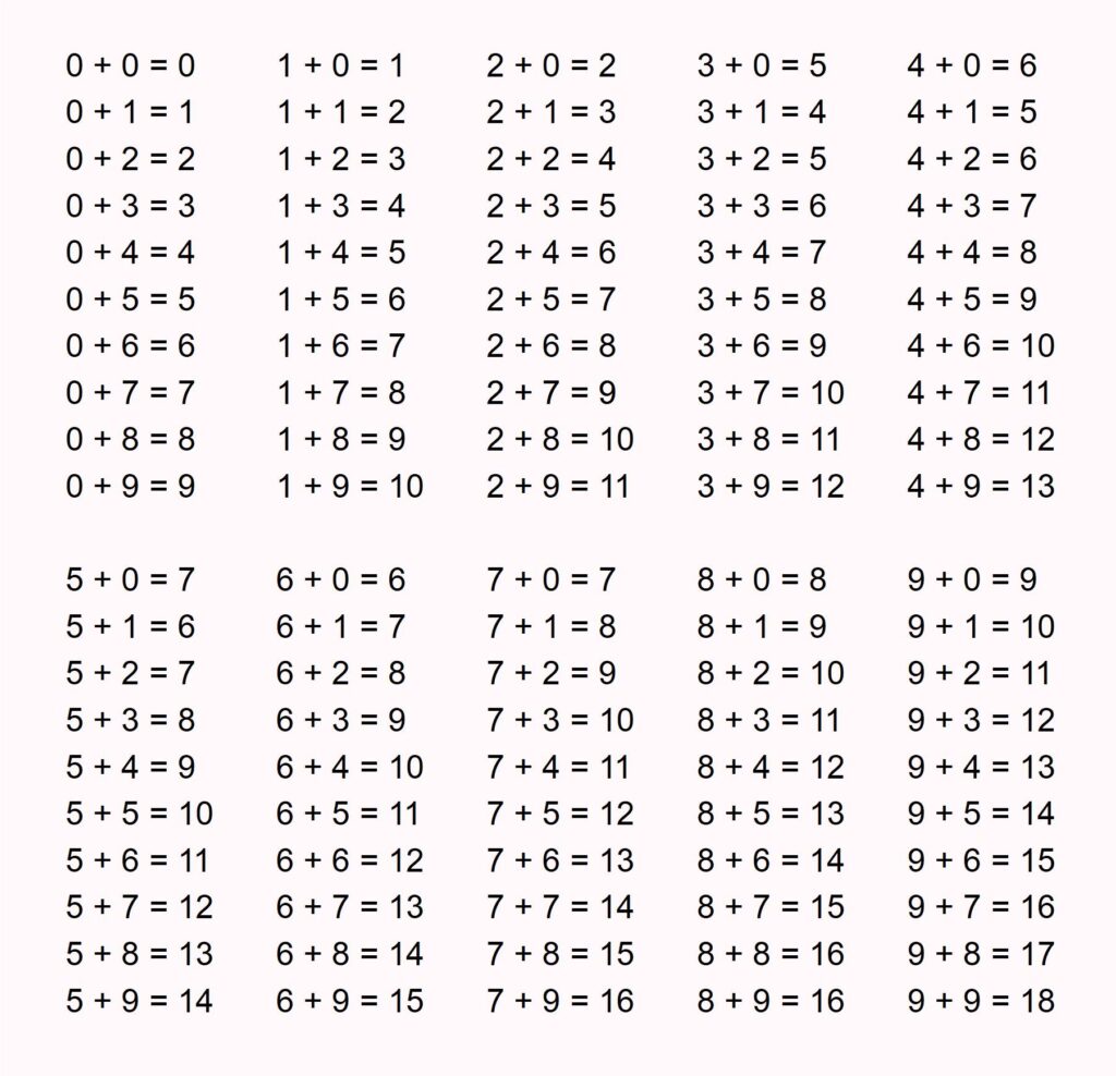
When people claim that the statement “One plus one is two.” is absolutely true, they often mean: “\(1+1=2\) is written in that list. So the equation must be correct!”
That the sequence of symbols \(1+1=2\) appears in the list is, by human judgment, hardly disputable. But what have we actually achieved with that? If we limit ourselves to judging the correctness of \(1+1=2\) only by whether this sequence of symbols appears in the list or not, then we indeed have a (quite) obviously correct sequence of symbols before us—but one that is meaningless so far. If we deliberately ignore the way in which the addition of numbers manifests itself in the real world, we may be right, but we lack relevance. With such an argument, we cannot justify that mathematics is correct (or perhaps even true), but only that a particular sequence of symbols appears i a list.
We can only add things that we can also count.
Here is, of course, an incomplete list of things that we cannot count:
rain, fun, catle, leisure time, courage, wood, snow, thunder, lightning, cheese, equipment, tea, traffic, underbrush, homework, trash, music, staff, luggage, baggage, clothing, research, livestock, sand, milk, oil, honey, weather, wool, broccoli, furniture, work, butter, news, dust, iron, gold, meat, money, love, happiness, heat, thirst, pasta, electricity, knowledge, and so on.
For these cases, \(1+1=2\) does not hold!
Normally, ‚time‘ has no plural. At times we sometimes need more time, but at no time can we need more ‚times‘. Even though we can have good times, we still can’t add them – it just doesn’t add up. Nevertheless we can add newspapers, and when we want to multiply 2 newspapers by 3, we write ‚2 times 3‘, but ‚The Times‘ is at all times treated as singular, even though it’s sold many times every day to people who don’t have time anymore since they read ‚The Times‘.
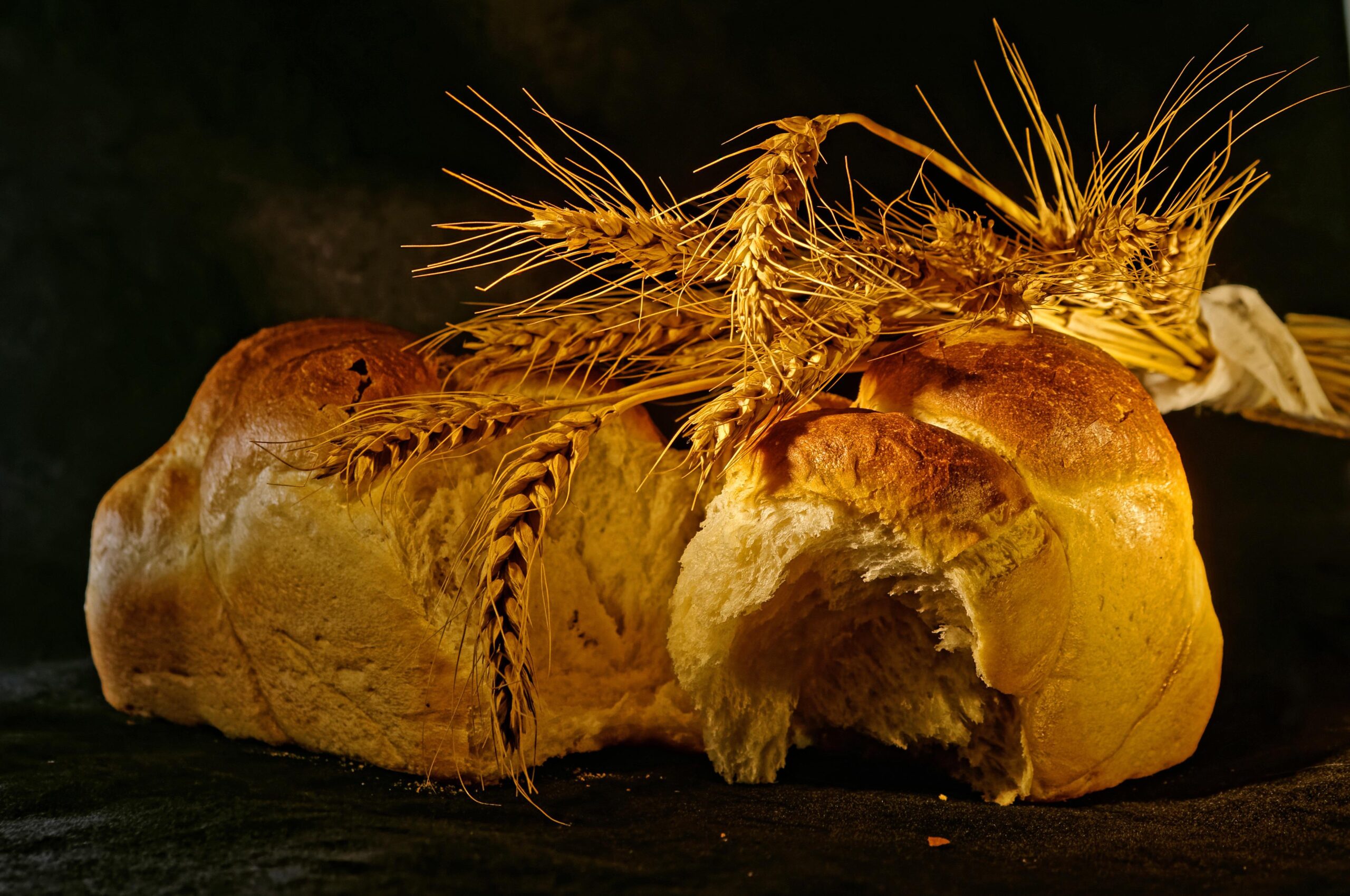
Bread – in the sense of a foodstuff – does not have a plural form. You need loaves of bread to be able to count and add up bread. But a bakery can have ‘breads’ in the sense of types of bread such as rye bread, sourdough bread, or baguettes. In German today, it is exactly the opposite: 2 breads (2 Brote) always means two loaves of bread, and if you want to distinguish between rye bread, sourdough bread, and baguettes, you need to use the term ‘types of bread’ (Brotsorten).
In English, ‚mathematics‘ is grammatically a plural form but is treated – like ‚Mathematik‘ in German – as uncountable and singular. The science that deals with counting, among other things, is itself uncountable, yet it includes subfields like geometry, which can be divided into multiple countable geometries (e.g., non-Euclidean geometries), or algebra, which as a branch of mathematics is uncountable but deals with algebras (e.g., Boolean algebras or Lie algebras).
As we can see, the validity of \(1+1=2\) depends on temporal, technical, linguistic, cultural, etc. contexts and does not apply in itself.
Fun fact: In Japanese, most nouns do not have a plural form. So does \(1+1=2\) not apply in Japan?
Let’s return to the first image: most people see two elephants on the left being added together, resulting in the same two on the right. In fact, however, the identical graphic appears four times in this image. Since we take into account that we cannot add the same elephant twice, we interpret the two identical graphics on the left as two different elephants, and on the right we do not see two more elephants or two representations of one elephant (after all, we are presented with two identical graphics), but rather another representation of the same two different elephants on the left.
This is a good example of how we humans tailor reality to fit our conceptual framework. So if \(1+1=2\) is true, it is because we humans want it to be true and, if necessary, we even bend actuality to make it fit.
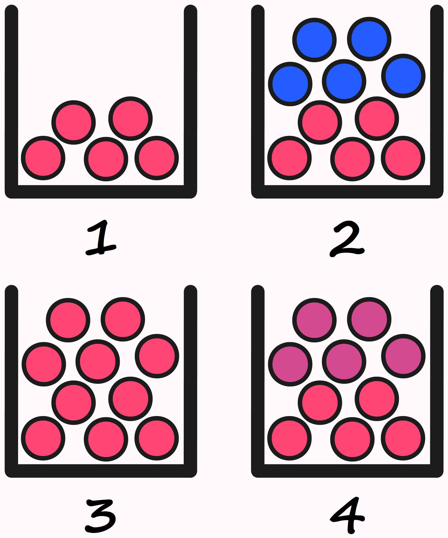
In which of the boxes are there \(5\) red balls?
Certainly, all boxes contain at least \(5\) red balls.
In the second box, there are \(5\) red and \(5\) blue balls. This raises the question of whether it makes sense to state the number of certain kinds of objects while leaving out the number of others. If someone asks for the number of balls in Box \(2\) and receives the answer, “There are \(5\) red balls in Box \(2\),” most people would probably imagine the situation in Box \(1\), not in Box \(2\).
We encounter such tricks and manipulations in everyday life as well — for example, when it is reported that there were \(30\) people at a counterdemonstration, but it is not mentioned how many people attended the demonstration being opposed. It makes quite a difference whether that number was \(5\) or \(50,000\).
The 555 red balls from Box \(1\) are — so to speak — still present in Box \(3\).
So, is it correct to say that there are \(5\) red balls in Box \(3\)? Or is that wrong?
Well, it’s not exactly wrong, since those balls are indeed included in Box \(3\).
It’s also true that they are not the only balls in the box.
It depends on what is being asked.
For example: if certain dangerous goods are transported by truck, the driver is required to carry \(2\) fire extinguishers. If the driver has \(10\) fire extinguishers and is asked during an inspection whether he has \(2\) fire extinguishers on board, answering “Yes” is both reasonable and factually correct.
Are there also \(5\) red balls in Box \(4\)?
That depends on whether we see two different colors of balls there, or whether we see \(10\) balls in two different shades of red.
This raises the fundamental question of how different elements of a set must be in order to belong to distinct subsets.
We cannot give a general answer to this question either.
In this case, it also depends on how clearly the observer perceives color differences — or on how precisely the particular screen displays color nuances.
As we can see, even counting up to \(5\) is not something that simply works automatically.
The meaningfulness of the number \(5\) depends, in each situation, on several different factors.
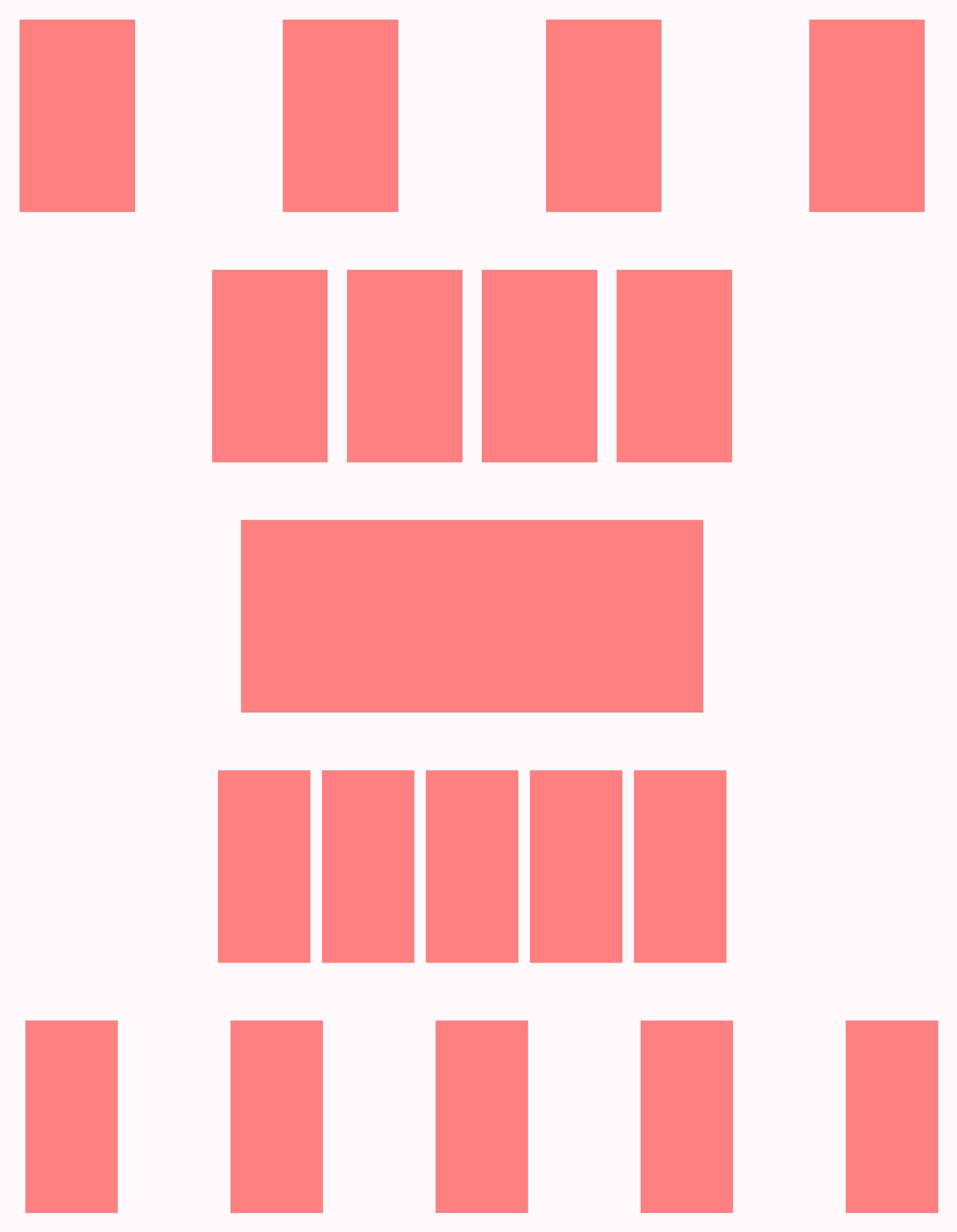
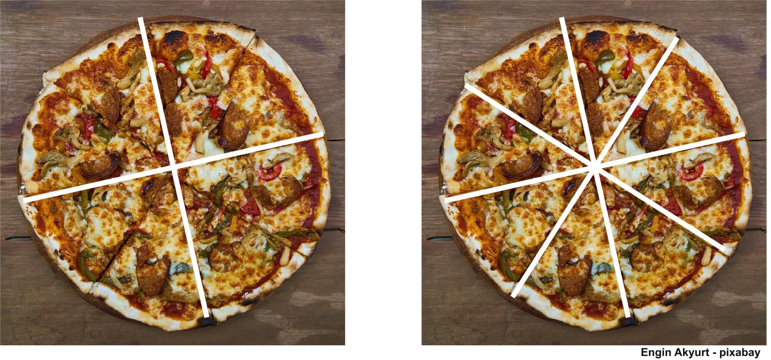
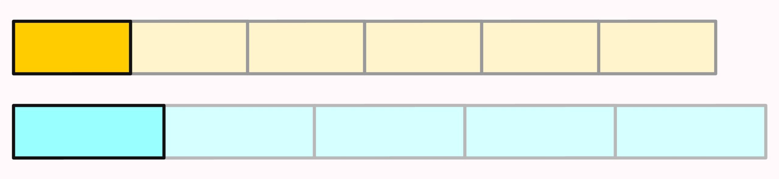
What happens in the image on the right can be imagined dynamically as follows:
\(4\) rectangles are pushed together horizontally to form one single rectangle.
Then this rectangle is divided into \(5\) smaller rectangles, which are then pulled apart horizontally.
This leads to several questions: When we push \(4\) rectangles together so that we can no longer distinguish them, do we then have one rectangle or still \(4\) rectangles?
When we divide one rectangle into \(5\) smaller rectangles but keep them together so that it still looks like a single rectangle, do we then have \(5\) rectangles or only one?
If we push \(4\) rectangles together so that there is no space between them and they therefore appear as one single rectangle, we can look at this one rectangle and say, “These are \(4\) rectangles.”
If we want to divide one rectangle into \(5\) equal rectangles, we must be able to imagine the \(5\) rectangles in order to divide it that way. Can we then have one rectangle in front of us and say, “These are \(5\) rectangles,” before we have actually divided the one rectangle into \(5\) rectangles?
After all, the \(5\) rectangles must at least potentially exist within the one rectangle for us to be able to divide it into \(5\) rectangles.
From this point of view, we can see a rectangle that was formed from \(4\) rectangles and that will be divided into \(5\) rectangles simultaneously as one rectangle, \(4\) rectangles, and \(5\) rectangles.
If we then change our mind and want to divide it into \(6\) rectangles instead, we can additionally see \(6\) rectangles within that one rectangle.
And how many rectangles can we see if we do not know how many smaller rectangles the given rectangle is composed of?
For us humans to perceive an object, we must form a unified whole from many sensory impressions and pieces of information. Which objects we see, and how many of them we see, usually depends on what we want to see. What we then count, and the numbers we obtain, also depend on our intention and our perspective. Thus, even the very beginning of mathematics is not given by god, but a human creation.
Wir können diesen „Schapernack“ (Leben des Prain) grenzenlos weiter treiben. Die nebenstehende Grafik ist aus dem Rechnen mit Äpfeln entstanden: Wenn wir \(4\) Äpfel haben, jeden in \(2\) Hälften teilen und dann eine Hälfte des ersten mit einer Hälfte des zweiten Apfels sowie eine Hälfte des dritten mit einer Hälfte des vierten Apfels zusammenfügen, gilt dann \(1+1=2\) ?
Die meisten Menschen stehen intuitiv auf dem Standpunkt, dass wir auf diese Weise nicht zwei Äpfel, sondern vier Apfelhälften addieren, obwohl „mathematisch“ gesehen \( \frac{1}{2}+\frac{1}{2}=1 \) ist.
We can take this way of thinking as far as we want. The illustration next to this text comes from arithmetic with apples: If we have \(4\) apples, cut each one in half, and then join one half of the first apple with one half of the second apple, as well as one half of the third with one half of the fourth apple, does \(1+1=2\) then hold?
Most people intuitively take the position that, in this way, we are not adding two apples but four apple halves — even though, from a “mathematical” point of view, \( \frac{1}{2}+\frac{1}{2}=1 \).
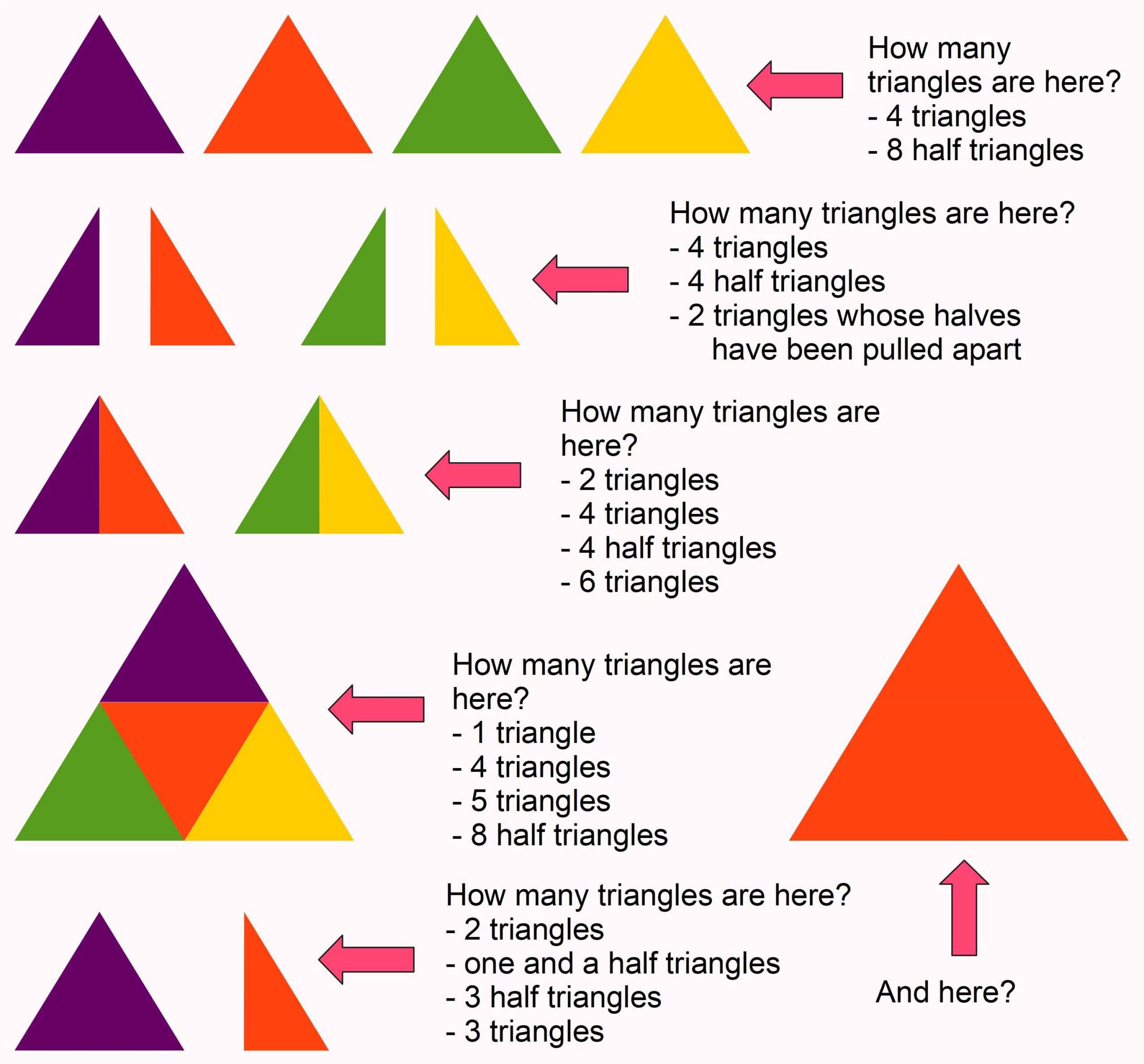
If we do the same thing with, for example, triangles, it becomes even funnier, because we can divide triangles in half in such a way that each half is still a triangle. If we then add four halves, that could either mean four halves, which equals \(2\), or simply four triangles, which equals \(4\). Or we can combine two halves into one triangle and then add the two triangles, which again gives \(2\) — but not because we added four halves, rather because we added two wholes.
If we divide a bread roll in the usual way into two parts, the top half is different from the bottom half. So they are not two identical halves. Can we still add them? Most of the time, the top parts are heavier than the bottom parts of the rolls. So if we add \(4\) top parts, the result would be a number greater than \(2\), wouldn’t it?
On the other hand, it is quite normal for halves to be unequal, since whenever we divide real objects into two parts, those parts are never exactly the same size. But since we want to calculate, we abstract from the concrete circumstances. So if, as in the case of the bread roll, we have two parts that are obviously different, we simply declare them to be equal. Question: Who’s the freak here?
Let’s imagine we have \(4\) tomatoes in front of us. We could group them in such a way that we can recognize the equation \(2+2=4\). Now let’s imagine we make a tomato salad out of these tomatoes and serve the salad to our guests. If we were then asked how many tomatoes are in the salad, we could truthfully answer “\(4\).” However, since we can no longer separate the individual tomatoes from the salad, these are \(4\) tomatoes that we cannot add. In that sense, it is not correct to say that addition can be applied to all “normal” everyday objects
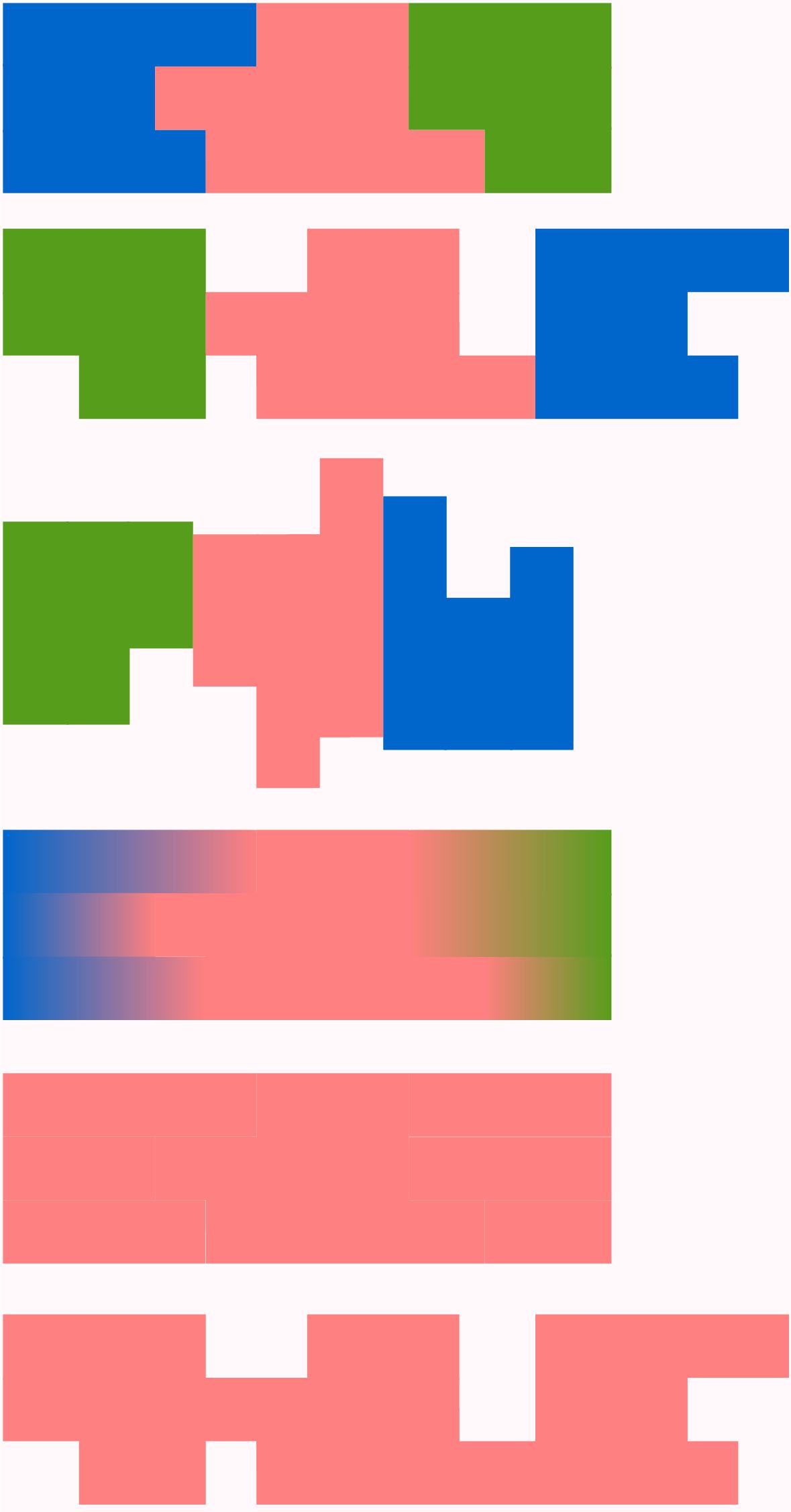
If three tomatoes are to be added together, most people imagine three tomatoes in a row that are equidistant from each other. Regardless of whether the tomatoes are swapped or in which order they are added together, the overall picture does not change. The three figures at the top of the right-hand picture behave quite differently. If we swap the order, there are still three figures, but the overall picture becomes wider and we intuitively realise that this is not what was actually meant by adding things together. If we rotate each figure by 90°, the whole becomes even narrower than before.
The three figures in the top picture can be distinguished from each other because they have different colors. But what happens if we color these figures differently, for example, by adding color gradients? Or if all figures have the same color, are there still three figures? Can we still add them then? Does that even make sense?
In my graphics program, the three figures at the top of the picture are actually 888 rectangles. But apart from me, no one knows that. Question: How many figures are there really?
And how many figures are at the very bottom of the picture?
Fractions
The fraction strips are in the Google Drive folder „Die besten Erklärungen der Welt“ and can be downloaded free of charge.
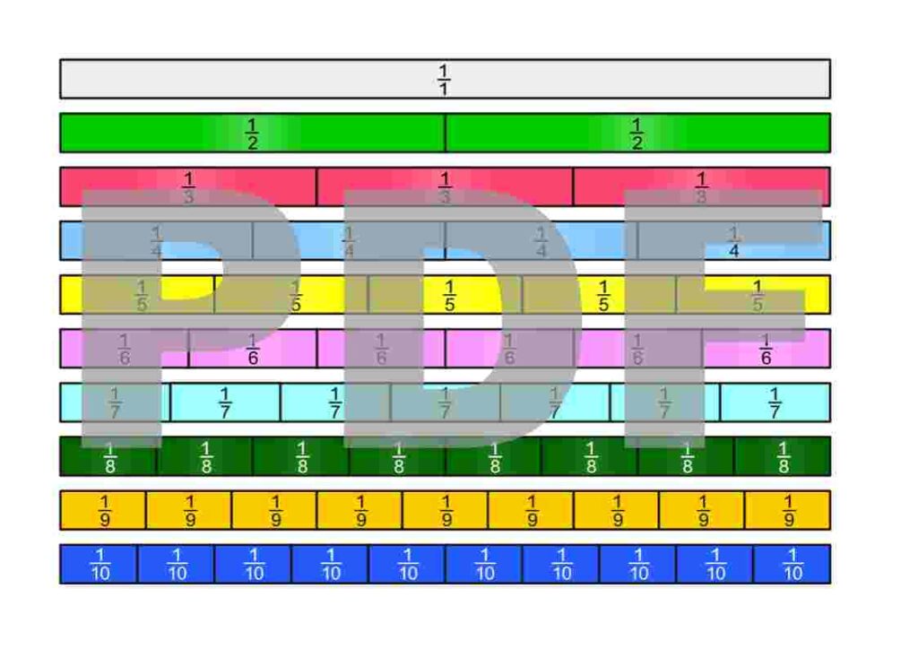
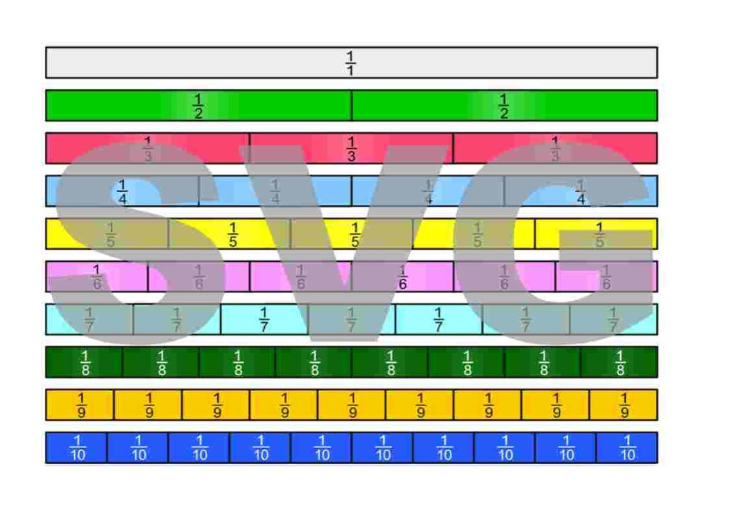
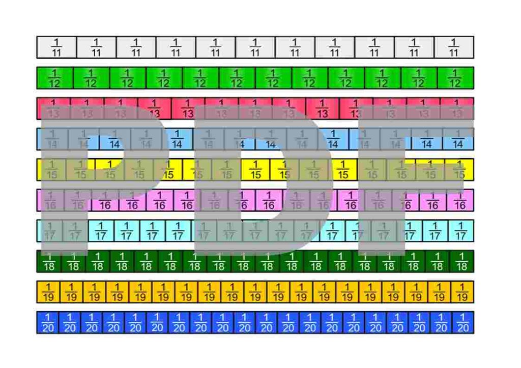
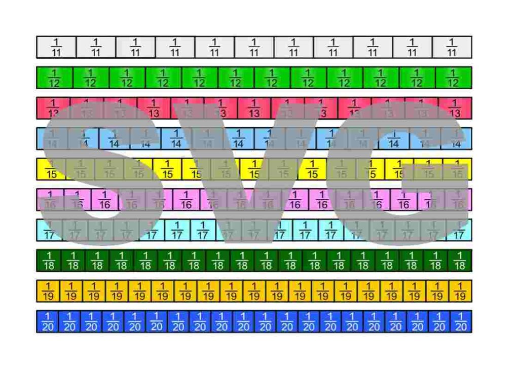
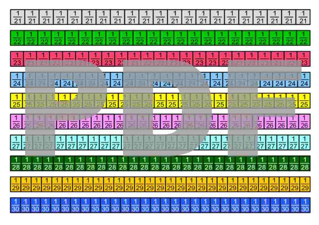
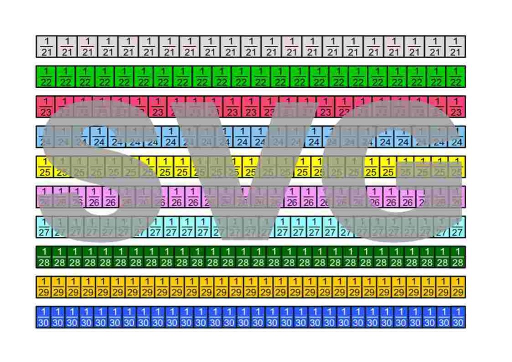
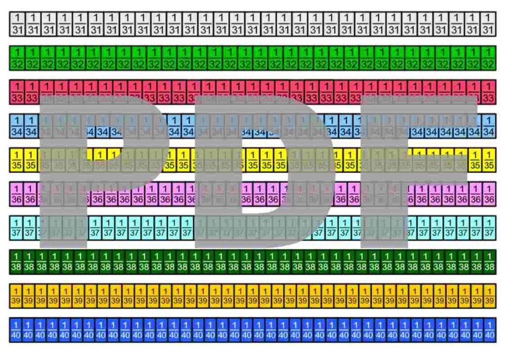
License Notice: I am deliberately releasing these materials under the most open license available: Creative Commons CC0 1.0 (Public Domain Dedication). This means you are free to print the fraction strips, modify them, include them in teaching materials, use them on YouTube or in books—even commercially. Attribution is not required.
Complete Course on Fraction Arithmetic (Definition, Expanding, Reducing, Common Denominator, Comparing, Adding, Subtracting, Multiplying, Dividing) Based on Fraction Strips
All operations with fractions are demonstrated and explained using the fraction strips. Additionally, intuitive explanations are provided for swapping numerators or denominators in fraction multiplication, cross-canceling in fraction multiplication, and the reciprocal rule in fraction division. The course is written for students. It can also be used alongside classroom instruction as a reference.
Fractions
Fractions – Introduction
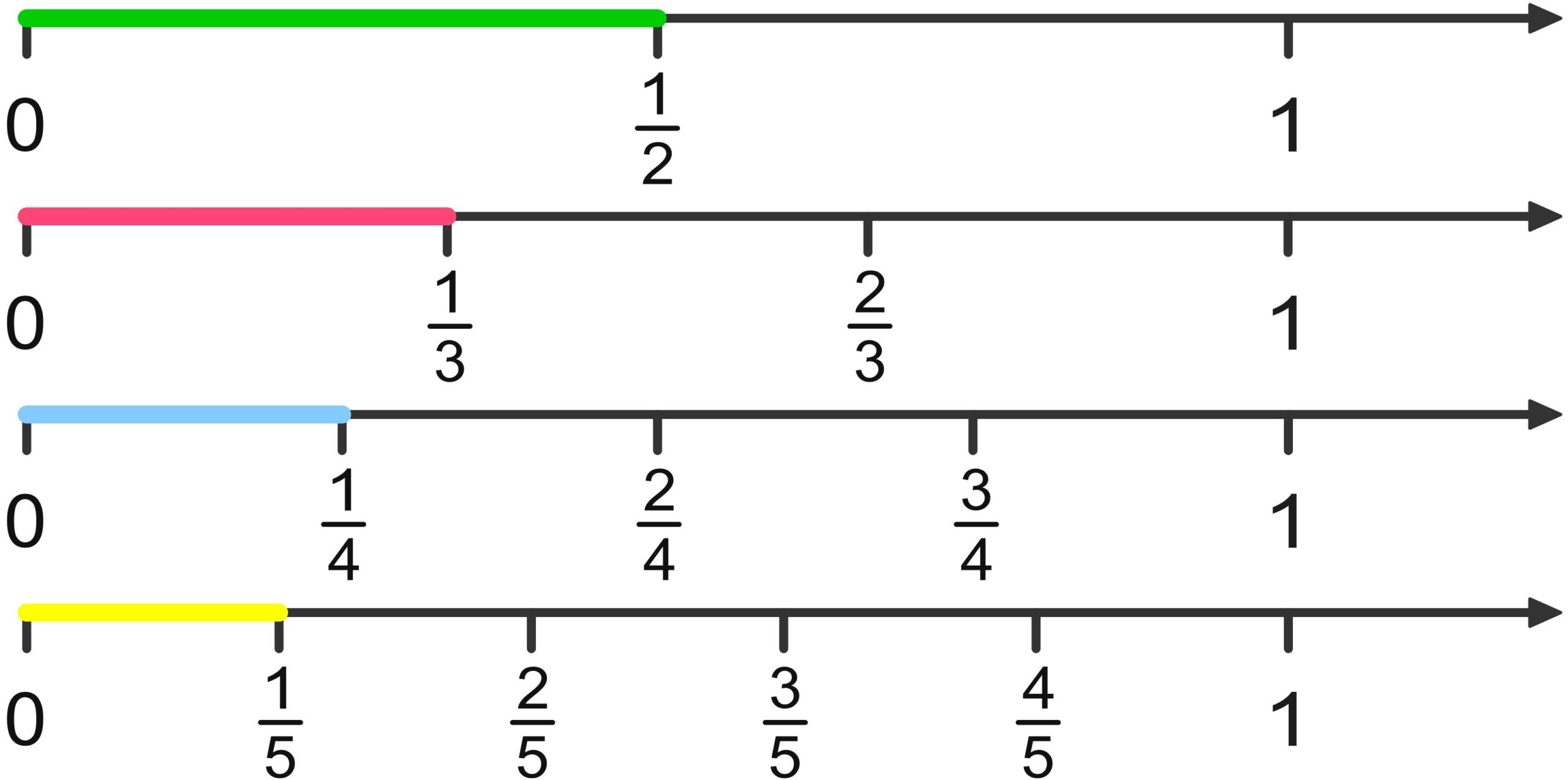
There are many ways to define what fractions are. To be able to work with fractions, we simply need to choose one definition and then derive all the properties of fractions from it. Here, we choose to view fractions as parts of a unit on the number line. The following PDF also introduces the first ways of expressing them.
Fractions can appear in many different contexts. Some of them are illustrated in the following PDF.
Expanding Fractions
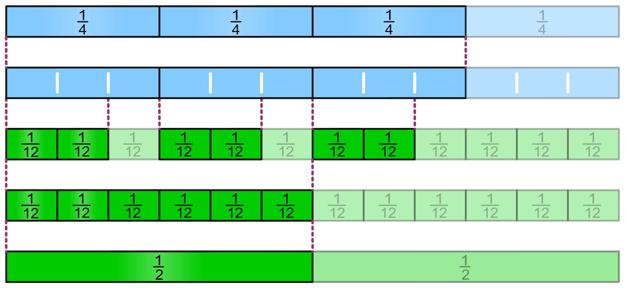
When we divide the parts of a fraction into smaller parts, we create a fraction of the same size. This process is called expanding. How we can visualize this is shown in the following PDF.
Further Questions
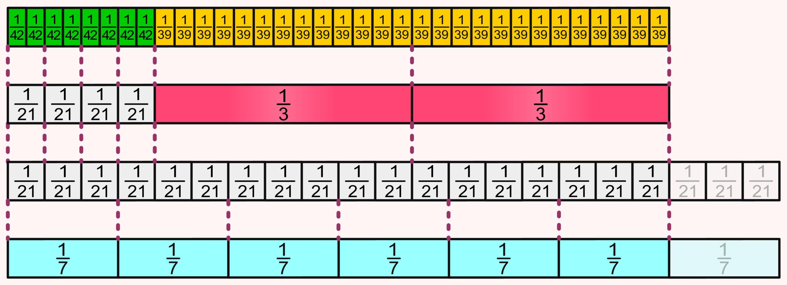
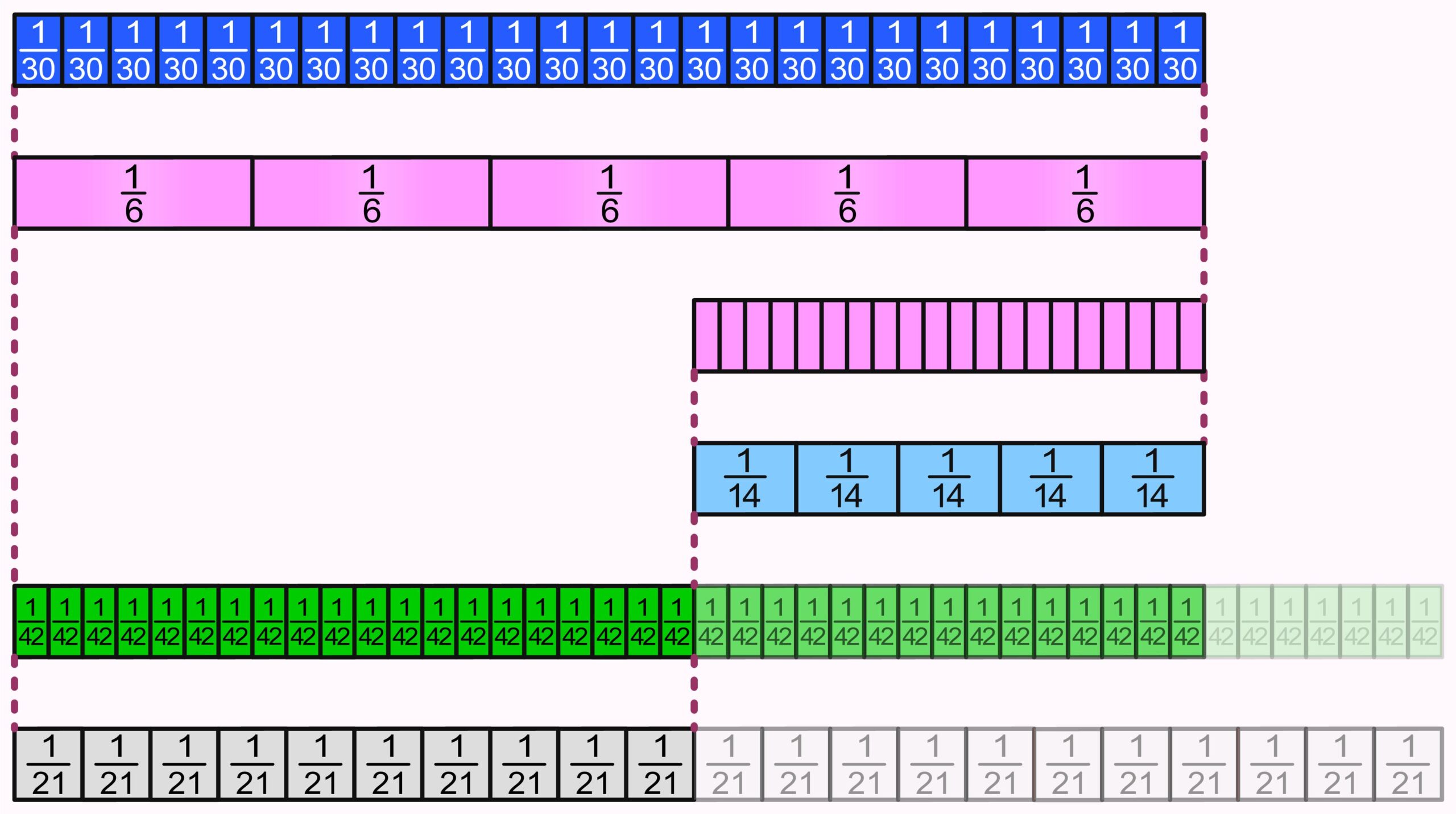
When we expand two fractions, we look for a common multiple of their denominators. If the denominators are relatively prime, the least common multiple is simply the product of the two denominators.
Common multiples can also be visualized with paper strips. Suppose we have several strips of length \(4\)and several strips of length \(7\). If we place the strips of length four and the strips of length seven side by side, eventually their total lengths will coincide: \(7\) strips of length four are just as long as \(4\) strips of length seven.
This also works with strips of other lengths.
Question: Which lengths must paper strips have in order to share a common multiple?
Partial Answer: As long as the lengths of the strips are integer multiples of some arbitrary unit length, they will also have common multiples.
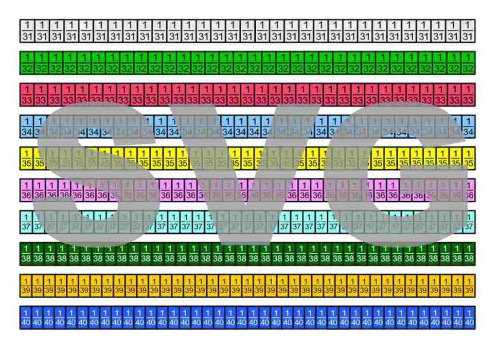
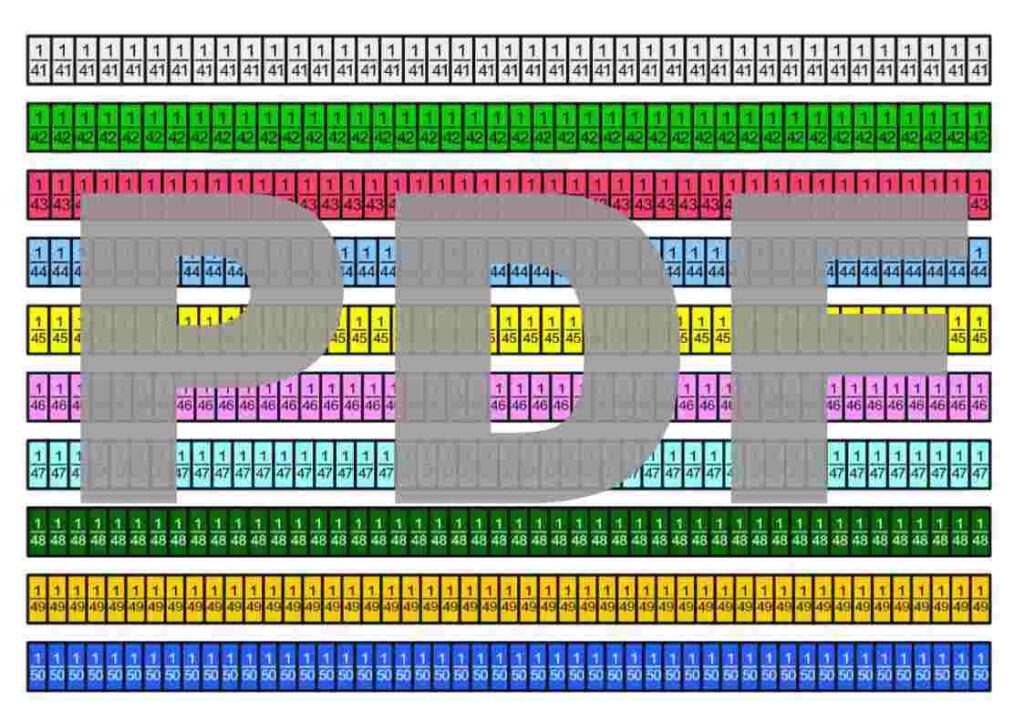
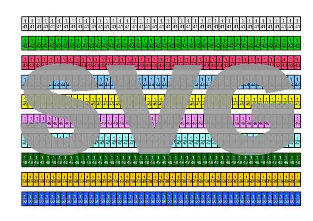
Question: But does this also work with non-integer multiples? For example, if one strip has a length equal to \(\frac{2}{3}\) of the length of a unit strip and another has a length equal to \(\frac{3}{4}\) of the length of that same unit strip, do these strips have common multiples? What about lengths \(\frac{37}{39}\) and \(\frac{38}{39}\) of a unit length? Or what about \(\frac{41}{43}\) and \(\frac{43}{41}\)? Can the difference between the two lengths tell us how many strips of each we must lay side by side to obtain equal total lengths?
Outlook: If the paper strips have lengths that are irrational multiples of a unit length, they will have no common multiple. However, no real paper strip can have a length that is exactly an irrational multiple of a unit length.
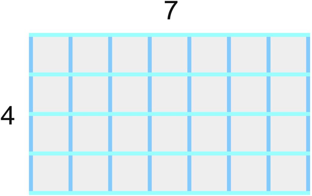
A similar issue arises from the division of a photo into rectangles or squares, as mentioned in the PDF. Of course, rectangular photos whose side lengths are integer multiples of some (arbitrary) unit can certainly be completely divided into squares.
Question: Can the areas of rectangles whose side lengths are arbitrary be completely divided into squares?
Question: Can the areas of rectangles whose side lengths are arbitrary be completely divided into smaller rectangles? Does the problem become simpler if the smaller rectangles have the same side ratios as the rectangle being divided? What happens in the case of rectangles with different side ratios?
Question: Can the areas of rectangles whose side lengths are arbitrary be completely divided into squares if the squares do not all have to be the same size?
Outlook: These questions can lead to the topic of tilings (or tessellations). In this area of mathematics, there are still several problems that remain unsolved.
Reducing Fractions
If the numerator and denominator of a fraction have a common factor, we can divide both the numerator and denominator by this factor without remainder. This produces a fraction of the same size. The fraction then consists of fewer, but larger parts. In the following PDF, we explore this visually using fraction strips.
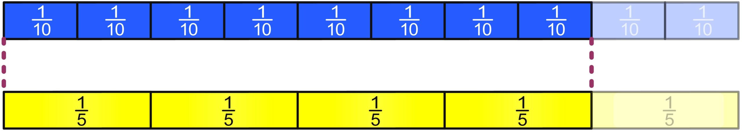
Least Common Denominator
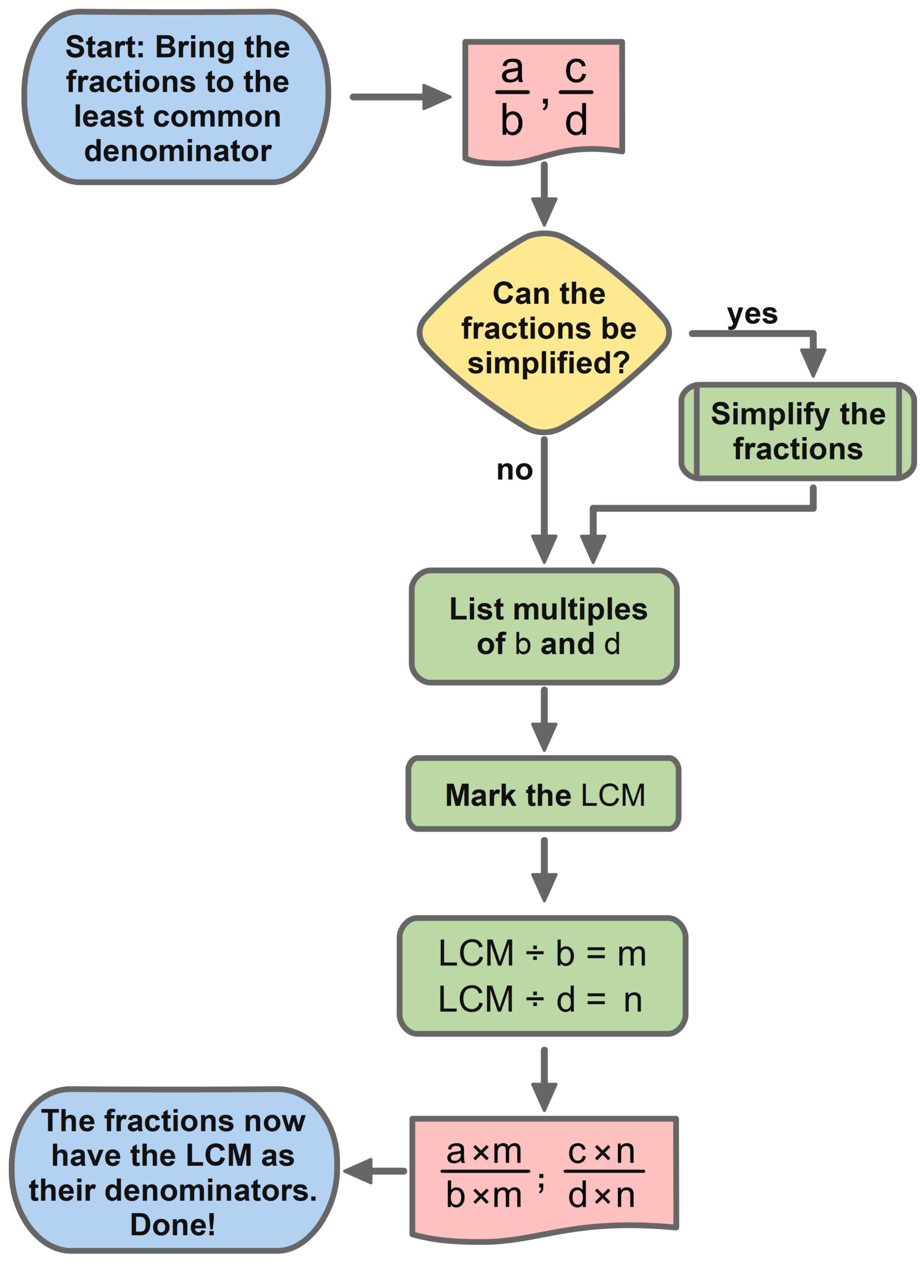
To add, subtract, or compare two fractions, we expand them so that they have the same denominator. One way to do this is to expand each fraction using the denominator of the other fraction. However, this can lead to unnecessarily large denominators. Therefore, fractions are usually expanded only to the least common denominator. The least common denominator is the smallest common multiple of both denominators. The following PDF shows how this is done and provides examples.
Comparing Fractions
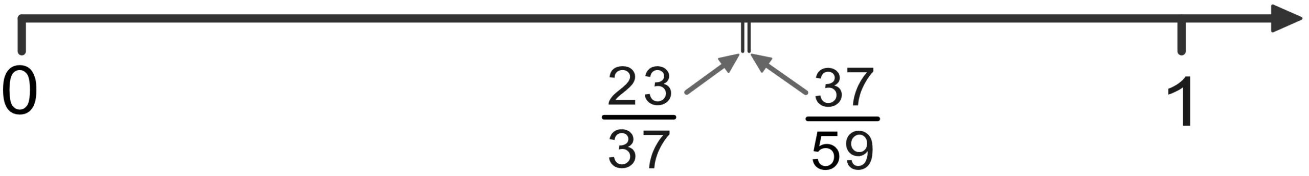
We humans can immediately recognize which of two given natural numbers is larger. For fractions with different denominators, this is not necessarily the case. However, if we expand fractions to have the same denominator, this becomes straightforward.
Adding fractions
At first glance, adding fractions may seem simple: make the fractions have the same denominator and then add the numerators. In fact, there are a few more steps involved: check the fractions for reducibility and simplify if necessary, determine the least common denominator, expand both fractions to the least common denominator, and then check again for reducibility and simplify if needed. The following PDF allows these steps to be followed using fraction strips—not only with the simplest fractions, but also with those that a typical student may encounter naturally. The fraction strips serve here as a standard model. The reasoning is: if adding fractions works with the fraction strips, this method can be considered valid and applicable to all fractions.
Further Questions
Question 1: Even when adding simplified fractions, it can happen that the resulting fraction can still be reduced. For which fractions does this occur? Under what conditions does it happen?
Note: In my view, there should be an elementary method to answer this question. However, I am not aware of one. Neither the internet nor AI could provide information, and my own attempts quickly became so complicated that I thought I must be making a mistake.
Question 2: The fraction strips serve here as a standard model for adding fractions. They help us understand how fraction addition works visually. We can reason that fraction addition could also be applied to other objects, as long as they are sufficiently similar to the fraction strips. What could this mean? Can we apply fraction addition to objects that are very different from the fraction strips? Fractions are often represented as circle segments. Does fraction addition also work with circle segments because the circle segments are sufficiently similar to the fraction strips? Or is it the other way around? Or something entirely different?
The addition of fractions can also be applied to frequencies. Are frequencies completely different from fractions?
Question 3: If we understand fractions as ratios, does it make sense to add them together? Since adding fractions assigns (at least) two fractions to a third—the resultant fraction—the question arises: Is there another calculation that meaningfully assigns two ratios—i.e., two fractions—to a third ratio? And what happens if we view fractions as proportions, or as the results of divisions, or as arithmetic instructions?
Question 4: If a whole is equal to $300, then (\frac{1}{2}) is equal to $150, (\frac{1}{3}) is equal to $100, and (\frac{1}{2} + \frac{1}{3}) is equal to $250. Instead of adding the fractions, we could also add whole dollar amounts here. Is it always possible to choose a whole in such a way that we can calculate with whole numbers instead of fractions? And if so, would that simplify anything?
Note: There is a similar concept in mathematics, namely percentage calculation. Here, the whole is always divided into (100) parts. (\frac{1}{2}) then consists of 50 of these parts, (\frac{3}{4}) consists of (75) of these parts, and (\frac{1}{3}) is approximately equal to 33 of these parts.
Question 5: Let’s assume that every fraction needs a whole in order to exist. For example, the fraction (\frac{1}{2}) needs a whole in order to denote half of that whole. Can we add two fractions if these fractions refer to different wholes?
Let’s assume that two fractions do not refer to the same whole, but to the identical whole, then we cannot add the fractions (\frac{4}{5}) and (\frac{3}{4}), for example, because (\frac{4}{5}) leaves only (\frac{1}{5}) left of the whole, and we cannot form the fraction (\frac{3}{4}) at all. Under these circumstances, what fractions can we form in order to add them?
Can we also add fractions if they do not refer to a whole, i.e., if they are simply abstract fractions? Does the addition make sense then?
We can also consider what a whole can be. If we put (\frac{1}{2}) kg of dough and (\frac{1}{3}) kg of dough in a bowl, is the amount of dough in the bowl a whole? And if so, would we still have a whole in the bowl if we added (\frac{1}{3}) kg of coal to the bowl?
Subtracting Fractions
In a similar way to how we add fractions, we can also subtract fractions. However, if we want to visualize this calculation using fraction strips, we have to change the direction of our thinking, and we cannot simply place the strips next to each other as we do when adding. The following PDF contains several worked-out examples in detail.
Multiplying Fractions
When we multiply fractions, we multiply numerator by numerator and denominator by denominator. But why, actually? In the following PDF, it is shown how we can understand this. In addition, the fraction strips illustrate why we can simplify „crosswise“ and why we can swap the numerators as well as the denominators when multiplying fractions.
Dividing Fractions
Dividing Fractions – Explaining the Reciprocal Rule – Measuring (Quotitive Division)

We divide by a fraction by multiplying with its reciprocal. This is called the reciprocal rule.
But why does the reciprocal rule work? To answer that, we need to ask ourselves what division really means. There are several ways to understand it:
Division is often understood as measurement. When we divide \(12\) by \(3\) , we can ask: How many times does \(3\) fit into \(12\)? The answer is \(4\), because \(3\) fits into \(12\) four times. When we measure the length of a distance, we proceed in a similar way: We take a measuring stick that is, for example, \(1\) meter long, and ask how many times this stick fits along a given distance. If the stick fits exactly four times, then the distance is \(4\) meters long.
If we want to understand the division of fractions as measurement, we can represent the fractions using fraction bars.
The PDF shows how fractions can be divided visually and how the reciprocal rule can be justified.
Didactical note: In the PDF, the visual explanation using fraction strips demonstrates how the validity of the reciprocal rule can be directly seen.
Moreover, the most difficult case is shown: both fractions have different numerators and denominators, none of the numerators and none of the denominators is equal to \(1\) , and the second fraction is greater than the first. While similar visual explanations exist, this is the only one that can handle the most complex case without relying on analogies.
Visual Explanation of the Reciprocal Rule – Video (German with English subtitles)
The reciprocal rule states: To divide by a fraction, multiply by its reciprocal. In mathematics, such a rule is not just stated; it is also justified. A purely visual justification is presented in this video.
Dividing Fractions – Justifying the Reciprocal Rule – Sharing (Partitive Division)
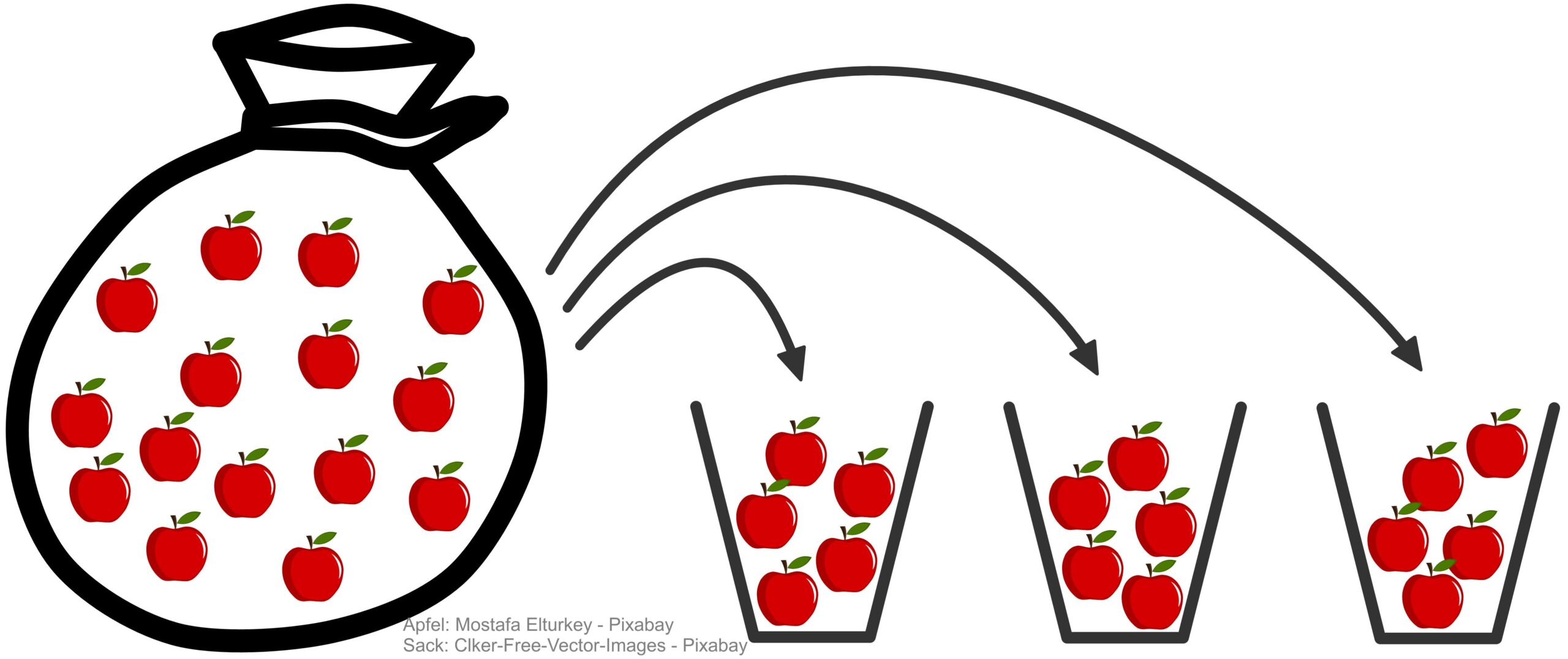
We can also understand division of numbers as „sharing.“ If we distribute \(15\) apples into \(3\) baskets, there are \(5\) apples in each basket. That is why \(15 \div 3 = 5\).
But how do we, for example, distribute \(\frac{4}{5}\) across \( \frac{2}{3} \) ? What could that even look like? The PDF shows how, by cleverly dividing areas, the justification of the reciprocal rule can be read off directly and visually. This brief presentation shows the „most difficult“ case: neither numerators nor denominators match, all are different from \(1\), and the fraction being divided into is smaller than \(1\).
Didactical note: The PDF presents the only existing visual justification of the reciprocal rule that is based on the idea of sharing (partitive division).
In this explanation as well, the validity of the reciprocal rule can be seen directly. There are indeed more general approaches — for example, distributing a certain amount of water among containers with different base areas, where the water level changes accordingly when poured — but only this explanation allows the numbers involved in the multiplication to be read off directly from the visual representation.
Algebraic Expressions and Equations
Associative and Commutative Law
The first two formulas that are usually introduced in mathematics class are these:
1) \(a+b=b+a\) and
2) \(a+(b+c)=(a+b)+c\)
The first formula is called the Commutative Law of Addition, and the second formula is called the Associative Law of Addition.
These formulas express something we already know from everyday life: No matter in which order we add things, the result is always the same.
In the video, we will look at how we can apply these formulas.
Further Questions
Question 1a) Why can we be sure that the Associative Law and the Commutative Law hold for all numbers? After all, there are infinitely many numbers, so it is impossible to test the validity of these laws for every number.
Possible answer:
When we add numbers in written form, we begin by adding the digits in the ones place. If the sum is greater than 999, we carry over the corresponding value to the tens place. Then we add all digits in the tens place, possibly carry again, and so on.
This means that, strictly speaking, we are always adding individual digits. Therefore, we could argue: If the Associative Law and the Commutative Law hold for all single-digit numbers, then they must also hold for all other numbers.
So we would only need to make sure—perhaps by checking through examples—that these laws are true for single-digit numbers.
Question 1b) Does the law \(a-b=-b+a\) also hold? Why?
Question 1c) Does the law \(a-b=b-a\) also hold? Why?
Question 1d) Does the Commutative Law of Addition also apply to repeating decimal numbers? Why?
Question 2: Why can we be sure that the Associative Law and the Commutative Law are true for all things? Or can these laws not even be applied to all things?
Possible answer: The video suggests that these laws apply to tomatoes, because as we can see, the laws “really” just mean regrouping tomatoes. And since we live in a world where regrouping tomatoes neither makes tomatoes disappear nor creates new ones, the laws presumably hold for all tomatoes.
But what about all other objects? One could argue that the laws also hold for all objects that are similar to tomatoes. Then we would only have to think about what “similar” is supposed to mean.
Question 3: In the video, it was stated that the commutative law applies to steps. However, it was not stated that the associative law applies to steps. So: Does the law also apply to steps? For example, how can one imagine \(3+(2+4)\) in connection with steps? Can one first take \(2+4\) steps and only afterward take the first \(3\) steps? According to the saying “You can’t take the second step before the first,” that is not possible. However, one could make paper strips corresponding to the length of one step, then place \(2+4\) “step lengths” on the floor first, and afterward place \(3\) paper strips in front of them. But is that still what is meant by “to walk”?
Question 4: For which things do the laws not apply?
Possible answer: The laws do not apply to things that cannot be added, such as justice or love. But are there things that can be added for which these laws still do not hold?
Another possible answer: One can also take the position that these arithmetic laws apply only to numbers, and that the question of what can be counted is no longer part of mathematics. In that case, however, mathematics would be nothing more than a board game with pieces that can indeed be moved according to clear and valid rules, but that have no meaning outside the playing board.
Question 5: In the video, it is shown how numbers can be substituted for variables. But can something else also be substituted for the variables? For example, can we substitute \(7+9\) for \(a\)? Or \(f+g\) ? Do the laws still hold then?
Possible answer: In general, in mathematical formulas (at least in those that occur in school mathematics), the variables can be replaced not only by numbers but also by expressions. The reasoning is as follows: by definition, an expression is a combination of numbers, variables, and operation symbols that can be evaluated. So if we already know that a formula holds for all numbers, then it also holds for all expressions, because evaluating an expression always produces a number for which the formula is already valid.
This context leads to the question: Do we actually know which expressions exist? In other words, if we say that all expressions can be substituted, it might be interesting to know which expressions there are in the first place. To put it briefly: in mathematics, new expressions are constantly being discovered or invented.
(Note: Even the question “Are expressions invented or discovered?” cannot be definitively answered.)
Therefore, we cannot know which expressions exist.
One could be satisfied with this answer — or continue asking: But if expressions are defined as something that can be evaluated, then expressions should always result in numbers, regardless of whether we know all expressions or not, shouldn’t they?
Possible answer: Not all results of calculations are numbers.
Question 6: What if the commutative law did not hold? Would we then have a different kind of mathematics? Would that lead to contradictions? What would be the problem?
Possible answer: One could define addition in a way similar to the moves of a knight on a chessboard. Then \(3+4\) could mean: first move \(3\) squares to the right and then \(4\) squares up. And if \(4+3\) then means to move first \(4\) squares to the right and then \(3\) squares up, addition would not be commutative.
Why Is a Negative Times a Negative Positive?
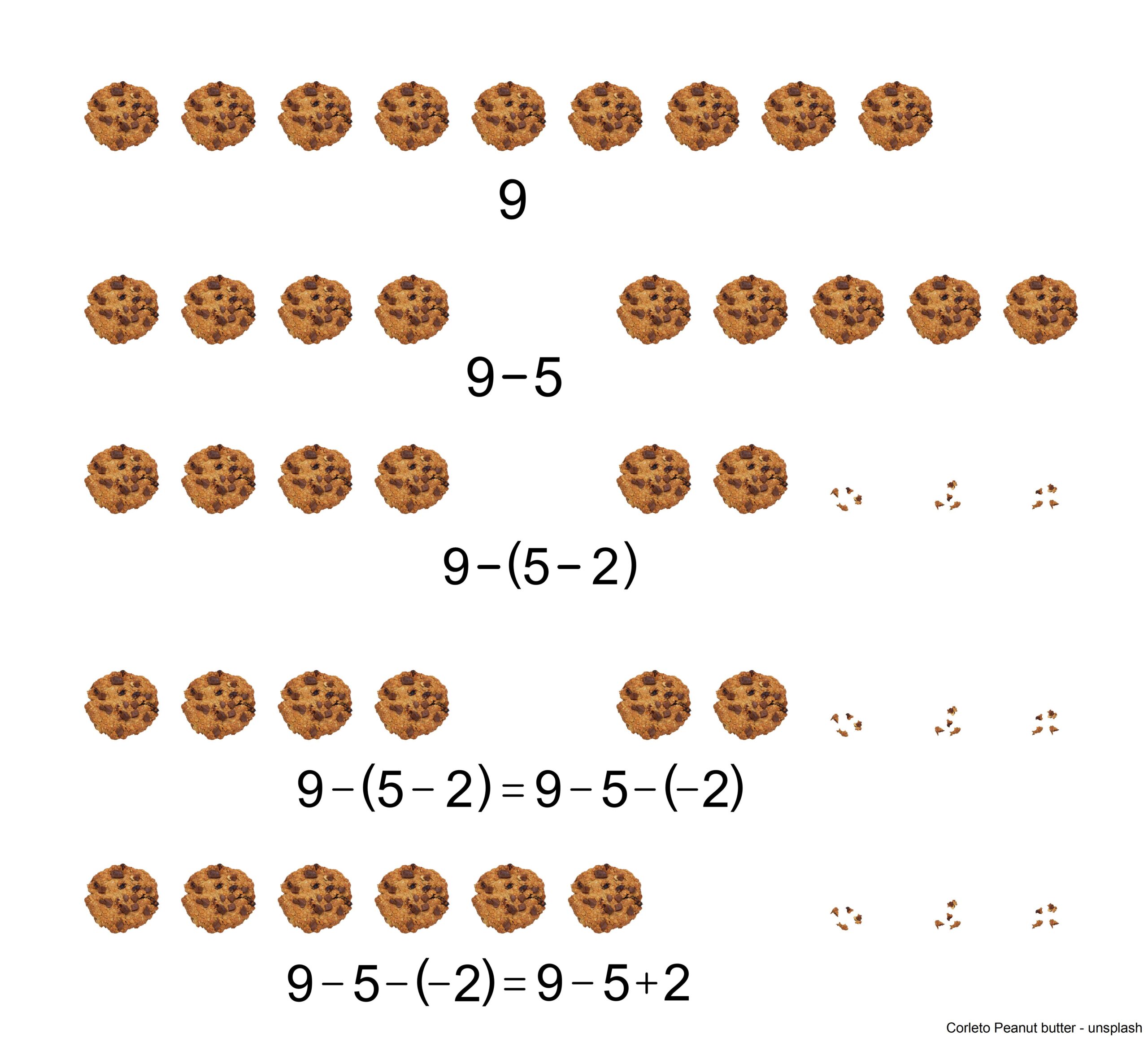
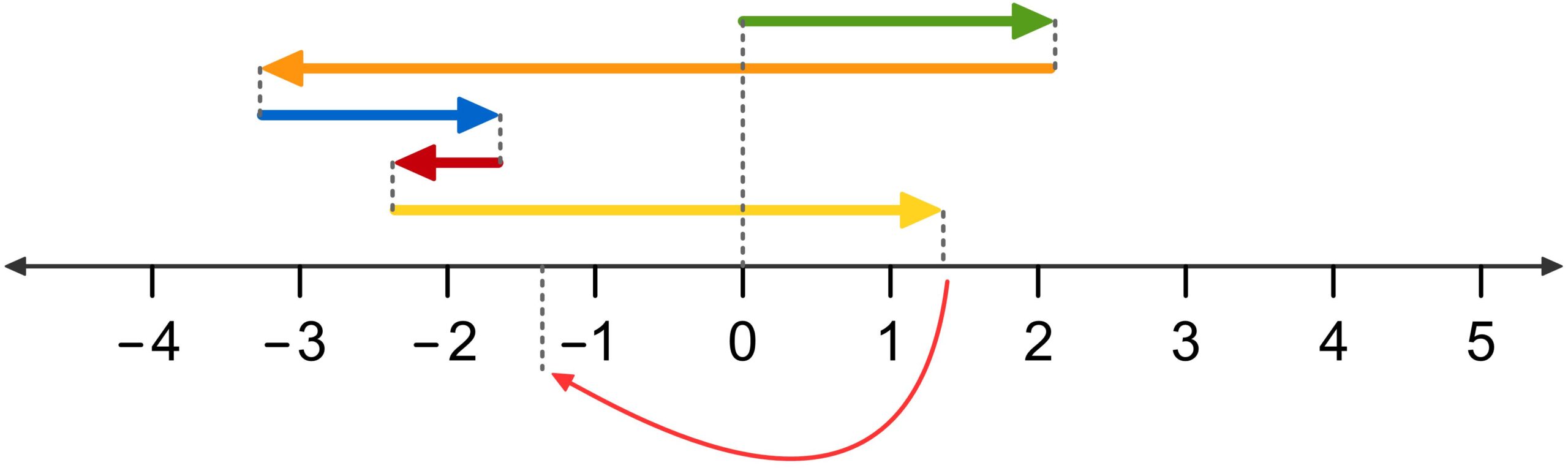
The rule that a negative times a negative equals a positive — for example, that \( -2 \times (-3) = + \; 6 \) — is the starting point of many more or less serious discussions about the correctness of mathematics. This is understandable, since this “negative times negative” seems to contradict the understanding of multiplication that we have known since elementary school. Back then, we learned that multiplication is a shorthand form of addition. For example, \(3 \times 4\) is either \(3 + 3 + 3 + 3\) or \(4 + 4 + 4\). In this context, an expression like \( (-3) \times (-4) \) simply does not make any sense.
The problem is indeed very deep: we cannot prove that “negative times negative” must inherently equal “positive.” However, we can show in certain mathematical models how such calculations make sense and also lead to correct results. In the following PDF, one topic is the number line as the standard mathematical model for arithmetic with numbers, and the other two models are more connected to everyday life: walking back and forth, and eating chocolate cookies. Yes, even for chocolate cookies, “negative times negative” equals “positive”!
In this video, a different explanation is presented: It is about the fact that every number should have an opposite number. The opposite number of a negative number must then be a positive number.
Further Questions
Not only the multiplication of two negative numbers must be justified, but also multiplication by \(1\) or \(0\).
The set of natural numbers \(\mathbb{N}\) is the set \({1, 2, 3, 4, \dots}\). (In some branches of mathematics, \(0\) is also included among the natural numbers.) In elementary school, we learned multiplication of natural numbers as a shorthand form of addition. For example, \(3 \times 4\) is either equal to \(4+4+4\) or to \(3+3+3+3\).
Question 1: It is defined that \(1 \times 4 = 4\). However, \(4\) is not added even once, but not at all. It is also defined that \(0 \times 4 = 0\). Here again, \(4\) is not added at all, but the result is not \(4\), it is \(0\). How can this be explained? Is this reasonable? Would there be any advantages to defining the results differently?
Question 2: When doing mathematics, one might get the impression that mathematics is the way it is because it has to be that way. However, in Question 1 it was said that multiplication by \(1\) and also multiplication by \(0\) are defined. But do these definitions have to be made? Or is there an argument showing that the results must be as they are? Could the results be defined differently? What would mathematics look like then?
(Didactic note: Even though it may sound unusual to many people, there are actually no standard answers to these questions! When you talk to mathematicians about this, the discussion quickly turns to axioms — some mathematicians believe that axioms must be as they are, while others believe they are stipulated.)
Expression Manipulation
Transformations of expressions provide a clear illustration of how the needs of highly able mathematics learners differ from those of other students. While most students try their best to imitate what was written on the board when transforming expressions, highly able mathematics learners ask questions that may seem bizarre to most of their classmates. Some of these questions may even be difficult for math teachers to answer. For example: What is an expression? What is a manipulation of an expression? In a manipulation of an expression, is an existing expression changed into another one, or is a new expression found in addition to an existing one? What makes a manipulation correct, and why? How can the reason for its correctness be understood intuitively? How can we prove that two expressions yield the same result for all numbers, even though there are infinitely many numbers? And why do we perform manipulations of expressions at all?
The following PDF does not provide complete answers to all of these questions. However, it shows several possible approaches one might take to gain a deep understanding of expressions.
Further Questions
Question 1: There are basically two ways to answer the question of what a manipulation of an expression actually is.
1) A given expression is changed. That means we have a single expression before the transformation, and after the transformation we have the same expression, but it now looks different.
2) For a given expression, another expression with the same result is found. One can imagine that for the given expression, there exists a set containing all expressions that yield the same result as this expression. From this set, one then selects a suitable expression.
In mathematics, it is in fact not determined which of these two views is the “correct” one. Therefore, when exploring these questions, it is quite likely that one will discover new mathematics in the process.
Question 2: When performing expressions manipulation, the goal is usually to simplify expressions. But can we always determine which expression is the simplest one? What does “simple” actually mean? What does it mean when one expression is simpler than another?
Question 3: Are there two equivalent expressions, but one cannot be transformed into the other expressions manipulation? The current state of mathematics on this question is: such expressions probably do not exist in the elementary context we are dealing with here. But this is not certain. If we do not specify at all how equivalent expressions are structured, how they are formed, or where they come from, then we also do not know which expressions are elements of the set of all expressions that are equivalent to a given expression.
Question 4: There are expressions whose value is always equal to 3. How can we show which expressions belong to this set?
Question 5: Is there a way to assign numbers to indicate the complexity of expressions? For example, we could define that the expression \(a\) has the number, because it is in its simplest form. The equivalent expression \(a+0\) could have the number \(1\), because one expression manipulation is needed to transform it into the simplest form. How could we proceed from there?
Question 6: Another way to evaluate the complexity of expressions (and thus perhaps to study the validity of expression manipulations in an ordered way) is to count the number of symbols. However, one quickly notices that an expression such as \(0+0+0+ \dots \) may contain many symbols but is still not perceived as particularly complex. Nevertheless, we probably cannot do without considering the number of symbols, since, for example, expressions consisting of only a single symbol cannot be very complex. What can be done?
Understanding Equivalent Transformations
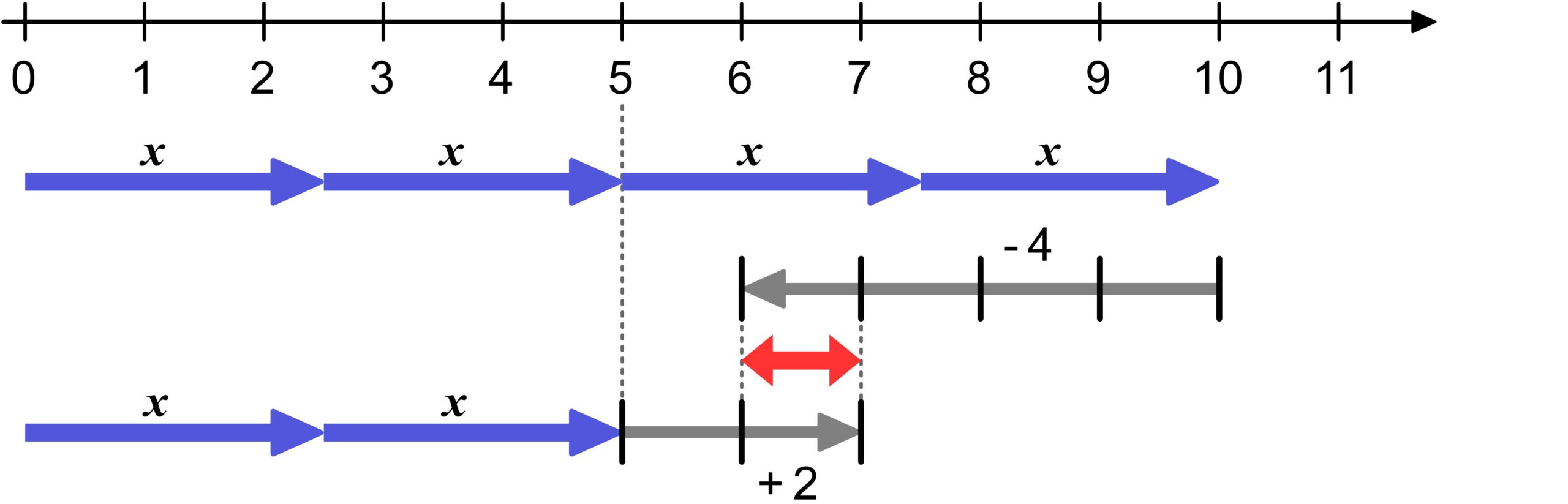
Just like expression manipulations, equivalent transformations can be illustrated on the number line. Interestingly, understanding them is much more complicated than actually performing equivalent transformations. We can observe this phenomenon in many areas of mathematics, and it represents part of the strength of mathematics: anyone can apply mathematics by substituting numbers into a formula without having to understand the reasoning behind the formula. However, the part of mathematics that involves striving for understanding is by far the more interesting one.
The pq-Formula for Quadratic Equations
The pq-formula is an important formula used to solve quadratic equations. In the video, we look at the formula itself, but not at how it is derived. Several examples are also worked through in which the pq-formula is applied. We observe that some quadratic equations have two solutions, while others have only one solution or no solution at all.
In this video, not only are the calculations shown, but it is also explained how to determine whether the pq-formula can actually be applied to a given equation. The following holds: the pq-formula is applicable when, by substituting values for p and q into the standard form of a quadratic equation, the given equation results. However, since this statement sounds rather cumbersome, the video does not go into it further; instead, the substitution process is demonstrated in a clear and visual way.
This also makes it easy to see which parentheses must be “carried along” when negative numbers occur in the given equation. Of course, in this video as well, all wording and notation follow the precise conventions used in mathematics. People who are used to the casual style common among YouTubers may find this demanding. Those who wish to learn how the calculations are “officially” stated and written will find what they are looking for here.
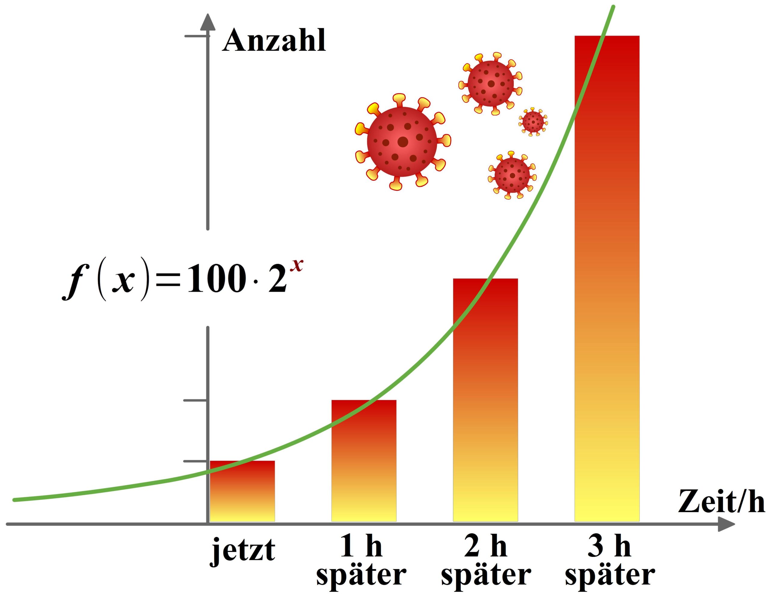
Exponential Function with Salt Dough
Exponential functions appear frequently in everyday life. We are practically surrounded by these functions. To demonstrate this fact in a very tangible way, this video models an exponential function using salt dough. This gives us a physical way to visualize what exponential functions are like.
And in the end, there’s even a striking insight: we can almost see for ourselves why any number raised to the power of \(0\) is always equal to \(1\).
Why is \(2^0=1\) ?
Just as multiplication is introduced as a shorthand for addition — for example, \(2+2+2=3 \times 2\) — exponentiation is first explained as a shorthand for multiplication, where, for instance, \(2 \times 2 \times 2 = 2^3\). As long as both the bases and the exponents are positive natural numbers, this causes no problem.
However, with \(2^1\), we already start to wonder. It is defined that \(2^1=2\). This still fits the definition of multiplication, since \(2=1 \times 2\). But when the exponent is \(0\), we must ask what \(2^0\) is supposed to mean.
Well, it is defined that \(2^0=1\), just as \(22^0=1\) and \( \left( \frac{1}{222} \right)^0 =1\). This may seem quite strange to many people. The following PDF explains why this definition was made and why it actually makes sense.
Differential and Integral Calculus
Derivative Without Limits
The differential quotient is the central concept of differential calculus. In this video, we explore how we can gain an intuitive understanding of what the differential quotient means. From a geometric point of view, it is about determining the slope of a tangent that touches the graph of a function at a single point. The difficulty is that, in order to determine the slope of a line — and a tangent is a line — we normally need two points, while the tangent shares only one point with the graph of the function.
Usually, this problem is solved by defining the slope of the tangent as the limit of the slopes of the secants. In this video, however, we take a completely different approach: we examine the slopes of the secants that are located in the neighborhood of the point of tangency. We then find that there is exactly one slope that is not a secant slope — the tangent slope. Thus, we determine the tangent slope by excluding all the other slopes. In doing so, we do not even need the concept of a limit.
Further Questions
The “trick” in differentiating without using a limit lies in answering the question of what a limit actually is. In school, it is usually assumed that the limit is the value that something approaches. In this video, however, we start from a different definition of the limit: the limit is the only number that cannot be reached by approximation.
Question 1: What are the advantages and disadvantages of both definitions of a limit?
Question 2: How could these definitions of a limit be written down in a formally exact way?
Question 3: Can we omit the proof that the number that cannot be reached is the only one of its kind? Could there be several such numbers?
We can apply a similar idea to sequences. For example, we say that the limit of the sequence
We can apply a similar idea to sequences. For example, we say that the limit of the sequence \( \frac{1}{2} , \frac{1}{3} , \frac{1}{4} , \dots \) — usually denoted simply as \( \big{\langle}\frac{1}{n} \big{\rangle}_{n \in \mathbb{N}}\) — is \(0\), because the terms of the sequence get closer and closer to \(0\).
The objection often raised in this context is: how can we be sure that \(0\) is indeed the limit if the sequence never actually reaches that number? One possible solution is to define the limit differently: in this case, the limit could be the greatest number that is smaller than all the terms of the sequence. We then say that this number is the greatest lower bound.
Question 4: Develop this idea of the limit further. For which kinds of processes would such a definition of the limit be advantageous, in your view?
Power Rule – Derivative
The power rule is used for differentiating power functions, and therefore also for all polynomial functions. As is customary in mathematics, the rule is first proven before it is applied.
The proof for natural exponents can be carried out by expanding a binomial. However, the power rule actually holds for all real exponents — a fact that is usually omitted in school mathematics.
For the general proof, one needs the chain rule and the derivative of the logarithmic function, but the amount of work required in writing it down is actually much less.
Chain Rule – Derivation and Visual Explanation
The chain rule is used to differentiate composite functions. In the video, the chain rule is introduced, a complete example is worked out, the formal justification is shown, and we also look at how we can understand the chain rule intuitively.
It must be explained why the product of the derivatives of the inner and outer function happens to equal the slope of the composite function. In addition, we consider why the derivatives are multiplied and not, for instance, added.
Fundamental Theorem of Calculus
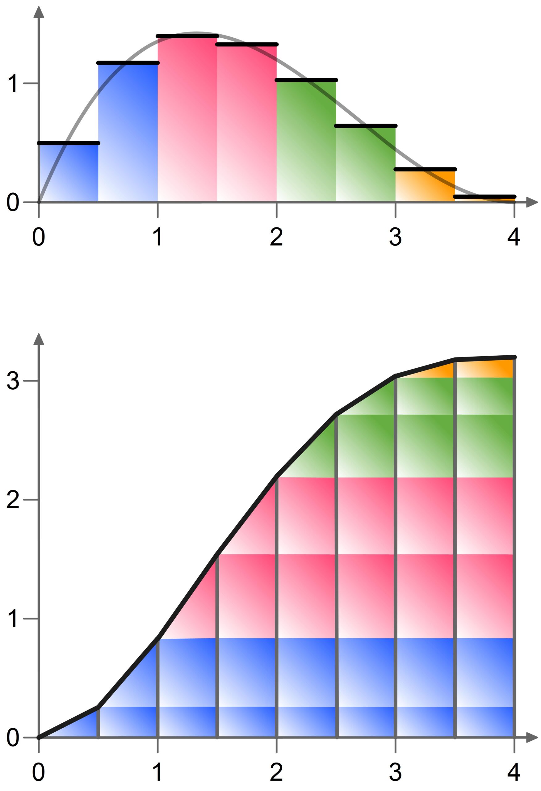
In a sense, the Fundamental Theorem of Calculus states that (under certain conditions) the derivative of an area function is exactly equal to the function values of the function whose area between its graph and the x-axis it measures.
Put more simply: Finding the area is the opposite of finding the slope, and vice versa. That might indeed seem surprising!
The formal proof of the Fundamental Theorem is short, but it does not offer any intuitive understanding of this relationship. Therefore, the accompanying PDF provides a visual explanation of why (under certain conditions) integration is the inverse operation of differentiation.
Under certain conditions, the Fundamental Theorem of Calculus can (in a somewhat simplified form) be understood as follows: An antiderivative can be used to calculate an area.*
However, an antiderivative, as the opposite of a derivative, has at first nothing to do with area. And yet, it works. How we can understand this relationship visually is shown in the video.
*More precisely: The area between the graph of a function f and the x-axis on the interval [a; b] can be determined by the difference of the function values F(b) and F(a) of an antiderivative F.
Improper Integrals
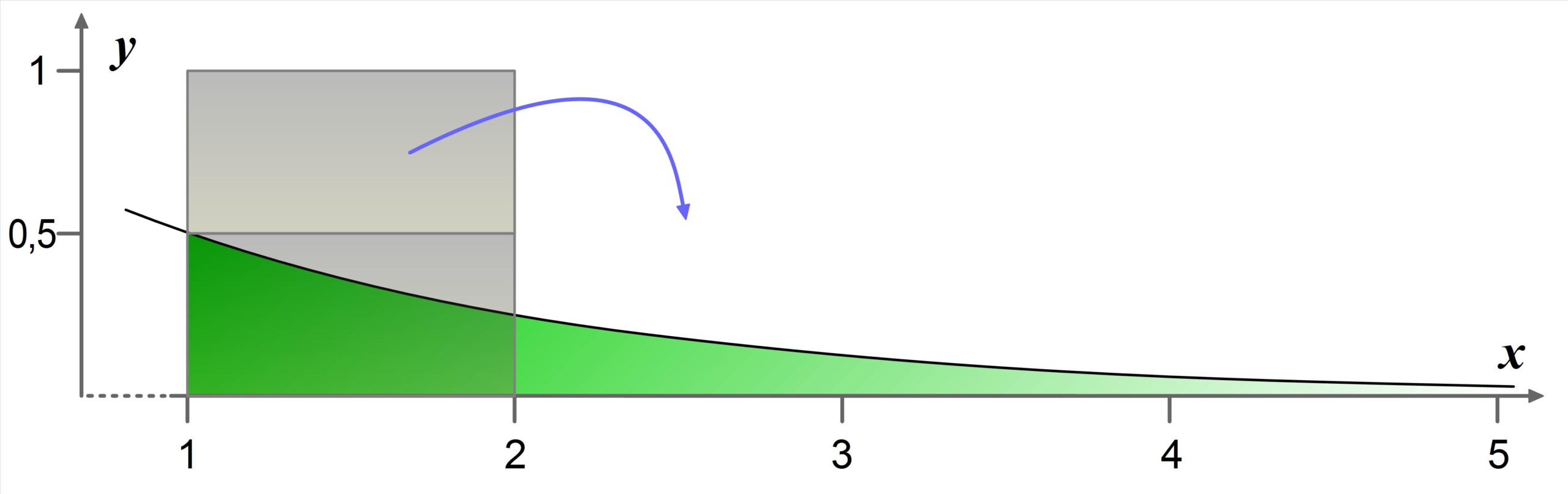
With improper integrals, one achieves the remarkable feat of having an infinitely wide area in front of us that nevertheless has a finite area. This usually defies common sense. All the more surprising is that there is an extremely simple explanation by which we can understand this seemingly paradoxical phenomenon.
Further Questions
In the context of improper integrals, we are dealing with two different processes. On the one hand, the green area under the curve can be understood as an area to which something is added infinitely many times. On the other hand, there is a finite gray area that is spread over an infinite width. Do such processes also exist in other mathematical or non-mathematical contexts? Perhaps for every sum with infinitely many terms whose result is finite, there is a finite quantity that can be distributed across the terms? Or more simply: Does one process always imply the existence of the other process?
In the text, the area of the gray square is larger than the entire green area. Is it also possible to have a gray area that is smaller than the entire green area? And if so: How large is the difference between these two gray areas? Can the difference be reduced? Can it be reduced to \(0\)?
It is \(\frac{1}{3}=0,\bar 3\). Here, we can understand \(0,\bar 3\) as \(0,3 + 0,03 + 0,003 + 0,0003 + \dots\). This is a sum that, despite having infinitely many terms, does not become infinitely large.
The sum \( \frac{1}{2} + \frac{1}{3} + \frac{1}{4} + \frac{1}{5} + \dots \) grows without bound, even though the terms themselves become smaller and smaller. From this arises, for example, the question of how „quickly“ terms must decrease for the sum not to grow without bound. Interestingly, in mathematics, there is currently no method to answer this question for all sums.
The questions posed here belong to the topic of convergence of series.
Probability and Statistics
What is probability?
IIn school, mainly two different concepts of probability are taught: the Laplace probability concept and the frequentist probability concept. Both of these concepts present considerable difficulties in understanding—apart from the fact that, according to the journal mathematik lehren, they are also circular. However, there is a very simple concept of probability that arises when the axiomatic probability is reduced to a school-level approach: probabilities are proportions. Furthermore, we can skip the discussion of whether this is the ‘correct’ probability, because we are dealing with proportions anyway—whether we are calculating the probability of drawing a winning ticket or determining the probability of an interval by integrating a density function.
Probability of Rain
In weather forecasts, one can hear statements such as: „The probability of rain today is 80%.“ The problem with this is that weather is not a random experiment, and therefore there cannot be a true probability of rain. In the video, we examine what such a probability of rain could mean. It does not mean that 80% of the area of the forecast region will receive rain, and it also does not mean that it will rain 80% of the time. Rather, it means that in the past, on 80% of the days with comparable weather conditions, it rained. Therefore, the „probability“ is actually a relative frequency. As can be read online, even this relative frequency is not always communicated to the audience. In the video, the discussion is not about whether this is actually the case, but about a possible explanation: this explanation is loss aversion, which can also be captured mathematically.
Bayes’ Rule – Illustration
Bayes’ rule is somewhat „strange“ because on the left side of the formula there is information that — at first glance — does not appear on the right side. In this video, it is shown using simple, intuitive methods how this can be understood.
Empirical Law of Large Numbers
Suppose we have a box containing one blue ball and one red ball. We randomly draw a ball, record its color, and then put the ball back. We repeat this process, drawing a ball each time, and continue in this way. If we carry out this procedure \( 100\) times, it is quite likely that we will draw approximately \(50 \) blue balls and approximately \(50 \) red balls. This „fact“ is the core statement of the empirical law of large numbers. But why is this the case? Certainly not because the „laws of chance“ demand it—as is sometimes grandiosely claimed. (And even if that were true, the question of „why?“ would still remain unanswered.) The shortest possible answer is: Because there are far more possible sequences with approximately \(50 \) blue balls than there are sequences with other distributions.
In the following PDF, the situation is explained in detail. It precisely defines what is meant by „far more possible sequences“ and also shows how the empirical law of large numbers can be understood using the Galton board. Furthermore, it demonstrates how, even without knowledge of combinatorics, the numbers of possibilities can be calculated for the first few trials using (extended) Pascal’s triangles.
The unique method of explaining the empirical law of large numbers presented in the PDF has the enormous advantage that the regularities can be recognized intuitively after only the first few trials. Therefore, it is possible to omit the usual (and often confusing) note that the empirical law of large numbers applies only to very, very many trials.
Relative Frequency and a Consequential Misconception
A widespread misconception is that the relative frequency of an event approaches the probability of that event as the number of trials increases. While it may well happen that after 100 coin tosses we obtain „heads“ approximately 50 times (i.e., the relative frequency of „heads“ is then close to the probability of „heads“), this does not have to occur.
In this video, it is demonstrated how much the understanding of probability theory suffers from this misconception, how this can be avoided, and what the reality actually is. It also shows how simple the underlying mathematics really is.
Why the Relative Frequency Does Not Have to Approach Probability
The claim that the relative frequency of an event must approach the probability of that event when a random experiment is repeated „many“ times is frequently (and incorrectly) cited as the central statement of the empirical law of large numbers. There are many formulations of this, some more incorrect than others. A completely false formulation can be found (at least, it could be found there), for example, on the pages of the MUED e. V. association (for members):
„This famous law of large numbers states that, in many independent repetitions of a random experiment—whether coin tosses, dice rolls, lottery draws, card games, or anything else—the relative frequency and the probability of an event must always come closer together: The more we toss a fair coin, the closer the proportion of ‚heads‘ approaches its probability of one-half; the more we roll dice, the closer the proportion of sixes approaches the probability of rolling a six; and the more we play the lottery, the closer the relative frequency of drawing the number 13 approaches the probability of 13. There is no disputing this law; in a sense, this law is the crowning achievement of all probability theory.“
Why This Is So Important:
To put it very briefly: If this law were correct in this formulation, there would not exist a single (repeatable) random experiment.
An example: Suppose we toss a coin randomly, so that the outcomes H (heads) and T (tails) are possible. Each outcome is supposed to have a probability of 0.5. Further, suppose we toss the coin 50 times and obtain T every single time. Then the relative frequency of T after the first trial was 1, after the second trial it was still 1, and the same after the third, fourth, and so on. In these first 50 trials, the relative frequency of T did not approach the probability of T at all.
It is often argued that the relative frequency and probability „approach each other in the long run“ or „after very many trials.“ But what is that supposed to mean? Does the coin, if it showed T too often in the first 50 trials, have to show H more frequently until the 100th trial to restore the balance? Or must the relative frequency only approach the probability by the 1000th trial?
No matter how we look at it: If relative frequency and probability must approach each other, the outcome of a coin toss could no longer depend on chance at some point, but would have to follow what the coin showed in the previous trials. In that case, the coin toss would no longer be a random experiment. One may debate what exactly randomness is, but it is certainly part of a random experiment like a coin toss that there is no law dictating what the coin must show.
The situation becomes even worse when, in an introductory course on probability, it is claimed that the probability of an event is the number toward which the relative frequency of the event “tends” if the random experiment is repeated sufficiently often. Apart from the fact that students have no clear understanding of what “tends” or “sufficiently often” means, they also cannot reconcile such a “definition” with their conception of randomness. This approach leads to the absurd idea that someone must tell the coin what to do, or that the coin has a memory and actively seeks to balance relative frequency and probability. As a result, the fundamental concepts of probability theory—namely, randomness and probability—become so contradictory that a student’s understanding of this area of mathematics is effectively impossible.
Unnecessary Statistics
One can read in any book on the introduction to probability theory that the relative frequency of an event does not have to approach the probability of that event, even after an arbitrarily large number of trials. All statistical methods that infer probability from relative frequency would be unnecessary if relative frequency were required to approach probability. The concepts of “convergence in probability” and the weak law of large numbers exist precisely because the relative frequency of an event does not analytically converge to the probability of the event. Why, nevertheless, incorrect mathematics is still taught in German schools is, for me personally, incomprehensible.
What Actually Holds
The weak law of large numbers holds. Applied to the case above, this law, stated in simplified form, means that the relative frequency does not have to approach the probability, but rather that the probability of it being close increases.
More precisely: We can ask how large the probability is that the relative frequency of T lies within a certain interval around the probability of T. Since the probability of T is 0.5, we can, for example, set the interval to (0.4, 0.6). The probability that the relative frequency of T falls within this interval becomes increasingly larger as the number of trials increases.
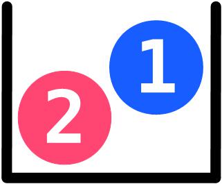
Let us consider the following random experiment: A box holds one blue and one red ball. One ball is drawn at random, its color is recorded, and the ball is then placed back into the box. After that, another ball is drawn at random, and so on.
If a red ball was drawn on the first trial, the probability of drawing a red ball on the second trial is just as large as on the first trial, namely 0.50.50.5. The same applies to other numbers of trials: for example, if after 99 trials 99 red balls have been drawn, the probability of drawing a red ball on the 100th trial is still 0.50.50.5. And this also holds if 99 blue balls were drawn before, or if any other combination of blue and red balls was obtained.
That means: the probability of drawing 100 red balls is just as large as the probability of drawing any other combination of blue and red balls. Therefore, after 100 trials, the relative frequency of red balls can be equal to 1. In that case, it is as far away as possible from the probability of drawing a red ball and not close to 0.50.50.5. The same reasoning applies for 1,000, for 10,000, and for any other number of trials. Thus, there is no number of trials—no matter how large—for which it must be true that the relative frequency of red balls lies close to 0.50.50.5. Therefore, as the number of trials increases, the relative frequency of red balls does not have to approach the probability of drawing a red ball.
The empirical law of large numbers is not by Bernoulli
It is often claimed that Jakob Bernoulli (1654–1705) was the first to formulate the empirical law of large numbers. However, that is not correct—at least not if one considers the common formulations of this law. Bernoulli did not write that the relative frequencies of an event A settle, for a sufficiently large number nnn of repetitions, at the probability of A. Nor did he write that the relative frequencies of an event A stabilize, as the number of trials increases, at the probability of A. And he also did not write that the relative frequencies of A must approach the probability of A as the number of trials increases.
This is, what Bernoulli actually wrote:
„Main Theorem: Finally, the theorem follows upon which all that has been said is based, but whose proof now is given solely by the application of the lemmas stated above. In order that I may avoid being tedious, I will call those cases in which a certain event can happen successful or fertile cases; and those cases sterile in which the same event cannot happen. Also, I will call those trials successful or fertile in which any of the fertile cases is perceived; and those trials unsuccessful or sterile in which any of the sterile cases is observed. Therefore, let the number of fertile cases to the number of sterile cases be exactly or approximately in the ratio \(r\) to \(s\) and hence the ratio of fertile cases to all the cases will be \(\frac{r}{r+s}\) or \(\frac{r}{t}\), which is within the limits \(\frac{r+1}{t}\) and \(\frac{r-1}{t}\). It must be shown that so
many trials can be run such that it will be more probable than any given times (e.g., \(c\) times) that the number of fertile observations will fall within these limits rather than outside these limits — i.e., it will be \(c\) times more likely than not that the number of fertile observations to the number of all the observations will be in a ratio neither greater than \(\frac{r+1}{t}\) nor less than \(\frac{r-1}{t}\).“ (Bernoulli, James 1713, Ars conjectandi, translated by Bing Sung, 1966)
German translation (slightly different):
„Satz: Es möge sich die Zahl der günstigen Fälle zu der Zahl der ungünstigen Fälle genau oder näherungsweise wie , also zu der Zahl aller Fälle wie \( \frac{r}{r+s}=\frac{r}{t} \) – wenn \( r+s=t \) gesetzt wird – verhalten, welches letztere Verhältniss zwischen den Grenzen \( \frac{r+l}{t} \) und \( \frac{r-l}{t} \) enthalten ist. Nun können, wie zu beweisen ist, soviele Beobachtungen gemacht werden, dass es beliebig oft (z. B. c-mal) wahrscheinlicher wird, dass das Verhältniss der günstigen zu allen angestellten Beobachtungen innerhalb dieser Grenzen liegt als ausserhalb derselben, also weder grösser als \( \frac{r+l}{t} \) , noch kleiner als \( \frac{r-l}{t} \) ist.“ (Bernoulli 1713, S. 104), in der Ausgabe: Wahrscheinlichkeitsrechnung (Ars conjectandi), Dritter und vierter Theil, übersetzt von R. Haussner, Leipzig, Verlag von Wilhom Engelmann, 1899)
What Bernoulli actually wrote is, in fact, correct and comes very close to the weak law of large numbers.
Computationally impossible
There are infinitely many possible situations in which the relative frequency of an event does not approach the probability of that event but instead diverges from it.
An example: Suppose we toss a coin randomly, so that we can obtain the outcomes T (Tails) and H (Heads). Both outcomes are assumed to have a probability of \(0.5\). Now, suppose we have tossed the coin \(100\) times and obtained \(50\) T and \(50\) H. Then the relative frequency of T is \(0.5\). If we toss the coin once more, we will either get T — in which case the relative frequency of T becomes \(0.\overline{5049}\) — or we will get H — in which case the relative frequency of T becomes \(0.\overline{4851}\). In both cases, the relative frequency of T moves away again from the probability of T. If, after obtaining T on the 101st trial, we continue to obtain T on subsequent trials, the relative frequencies of T will be as follows:
\(\approx 0.5098\), \(\approx 0.5146\), \(\approx 0.5192\), \(\approx 0.5283\), usw.
Thus, the relative frequency of T moves farther and farther away from the probability of T, which contradicts the so-called Law of Large Numbers.
Unusual Sequences
The empirical Law of Large Numbers is often justified by saying that unusual outcomes may occur, but they are so unlikely that they practically never happen. For example, in 30 coin tosses, the outcome HHHHHHHHHHHHHHHHHHHHHHHHHHHHHH is said to be very unusual and also unlikely, while the outcome HTTHTHHHTHTTHTTTHTTHTHHTTTTHT is considered much more normal and therefore more likely.
This is not only wrong because both outcomes have exactly the same probability, but also because we humans imagine the unusualness of certain outcomes into the outcomes themselves. In other words, the coin “knows” nothing about unusual results. Let’s look at an example:
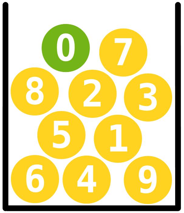
Let’s assume we have ten balls labeled with the digits from 0 to 9. The ball labeled 0 is green, and all the others are yellow. We draw ten times at random, with replacement and with order.
If we only pay attention to the colors, we would probably not consider the result

unusual. But if, upon examining the digits, we discover the following sequence

the sample would probably be regarded as unusual.
However, we can set entirely different standards if we wish: we might decide that a sample is to be considered unusual if its sequence of digits appears in the first decimal places of π. The sample
is ordinary, because it does not occur even within the first \(200\) million decimal places of π. The sample

is unusual, because it occurs at position 3,794,572. The sample

even appears at position 851 and is therefore extremely unusual.
Whether unusual or not, the probability of each sample is exactly the same, namely \[\frac{1}{10\,000\,000\,000}\]
What actually holds true
Let’s look at an example: We randomly draw one ball from a box containing two balls. One ball is blue, and the other is red. We draw several times, with replacement and with order.
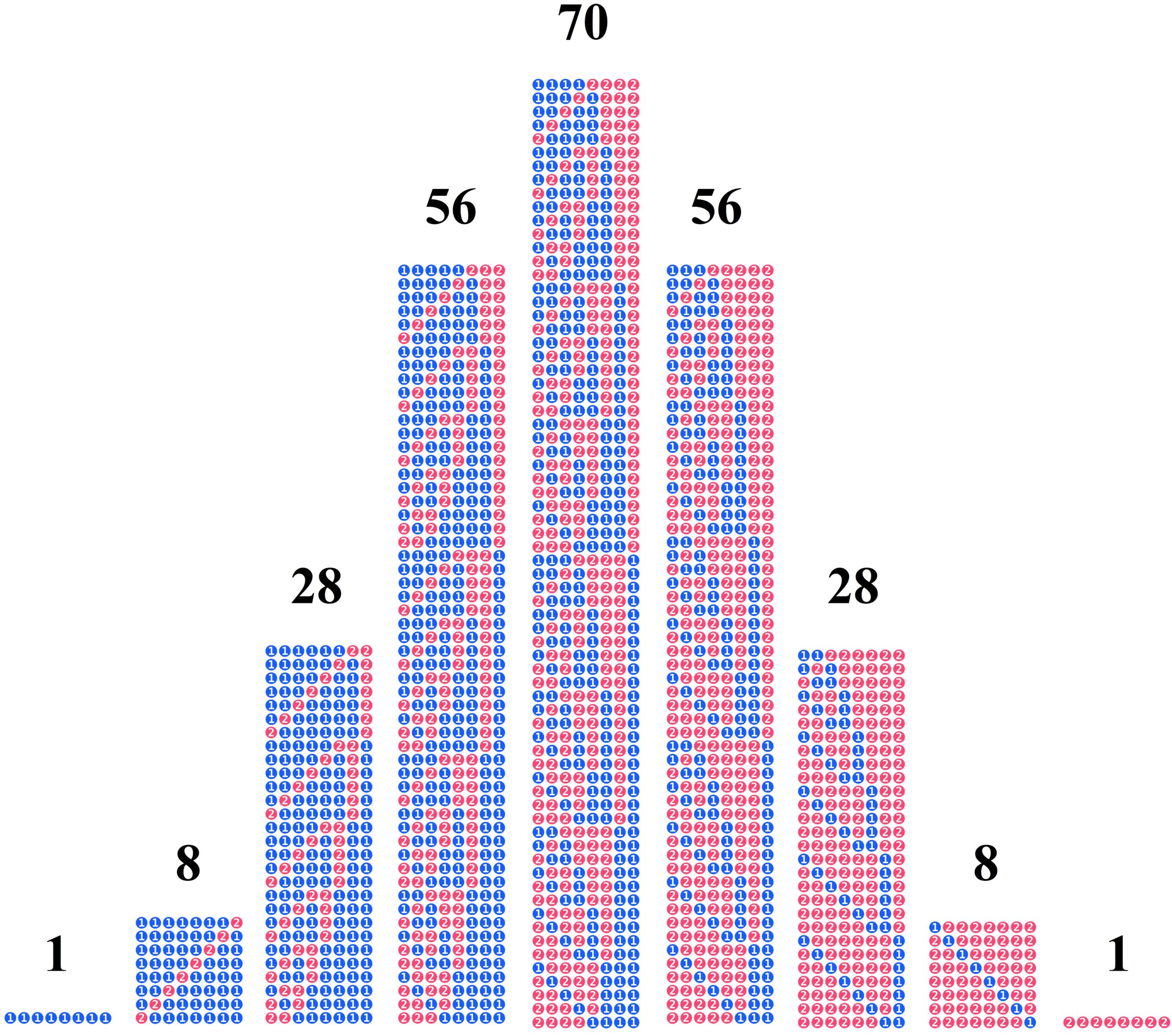
We will now focus on the numbers of red balls. In the following tables, these numbers are listed depending on the number of trials performed. For example, when drawing eight times, there are 56 outcomes with exactly 3 red balls.
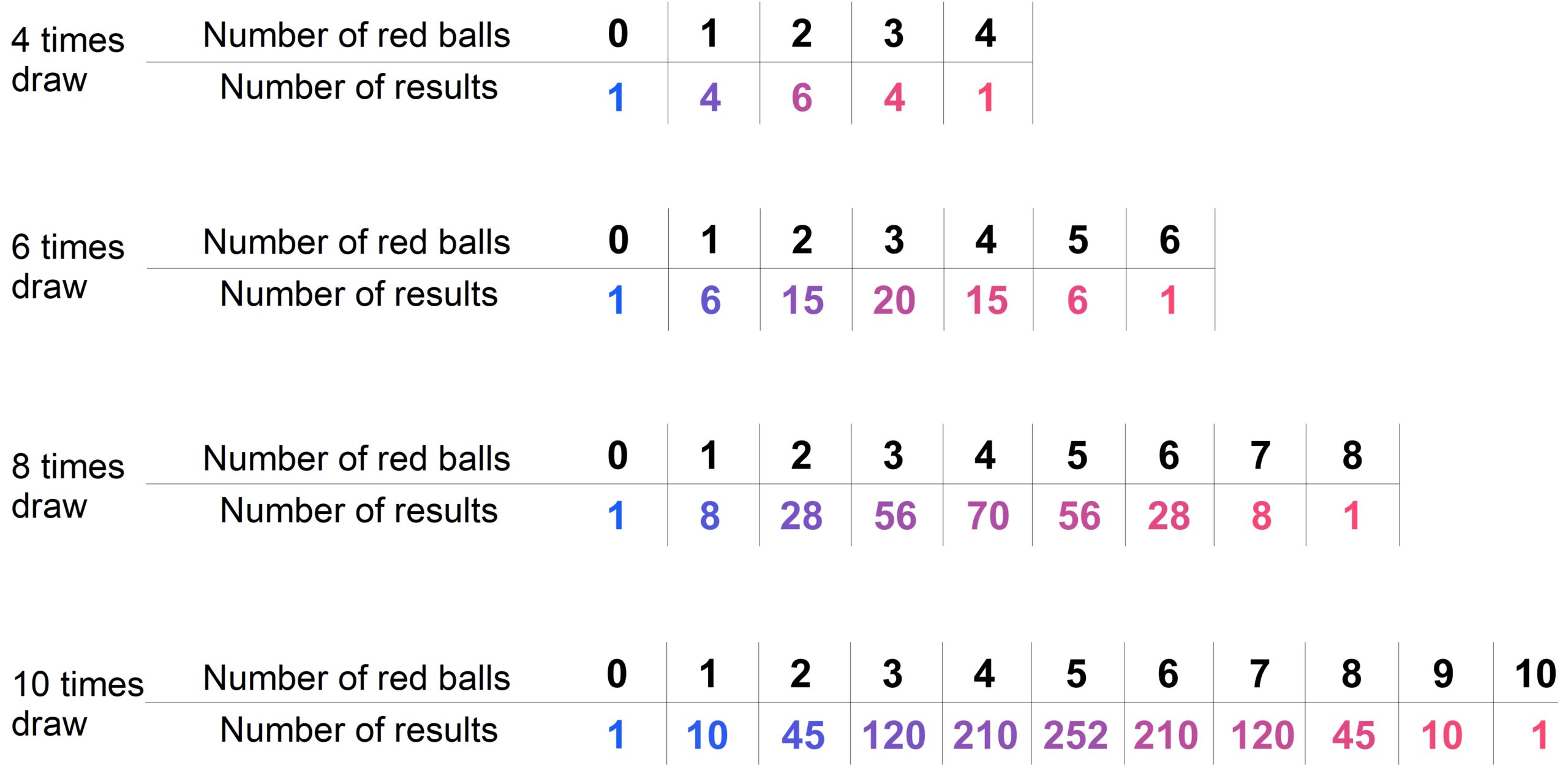
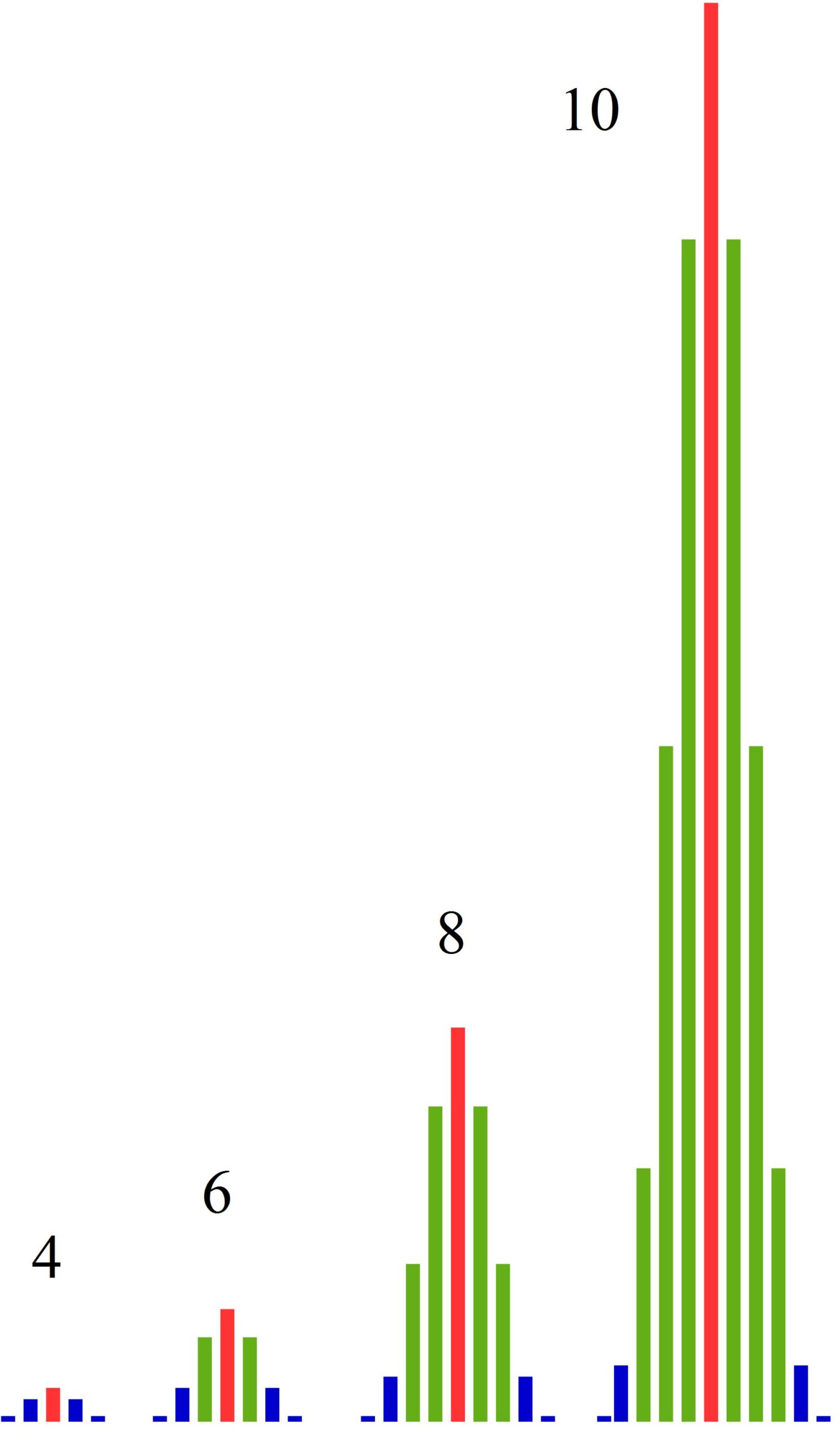
These numbers are represented to scale in the following bar charts. As we can see, with an increasing number of trials, the numbers of outcomes in the middle grow much faster than those at the edges. The more often we perform the experiment, the greater the differences become between the middle and the edges.
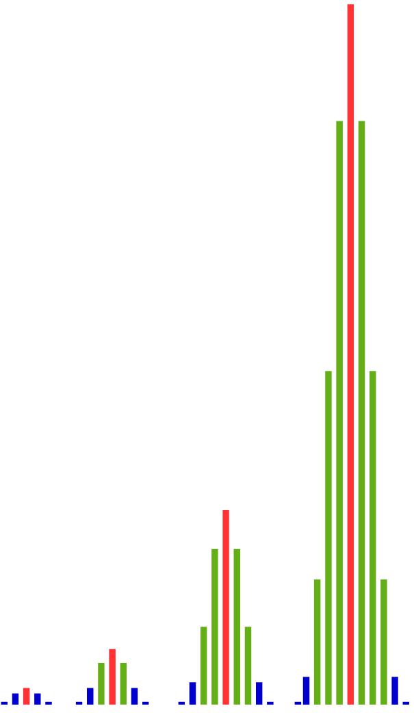
That means: There are simply far more outcomes with approximately 50% red balls than there are outcomes with much fewer or much more red balls. And the proportion of outcomes near the center becomes larger and larger as the number of trials increases.
We can observe this phenomenon also with other proportions of red balls in the population: If two-thirds of the balls in the population are red, we see a clustering of outcomes with about two-thirds red balls.
What we see here can be summarized—somewhat simplified, but not incorrectly—by the following statement: The relative frequencies of red balls are, in most outcomes, similar to the probability of drawing a red ball.
In statistical terms, this sounds like this: Most samples are similar to the population.
So if we flip a coin 100 times and get about 50 H, this is not because the relative frequency stabilizes, or because the coin strives for a balance between H and T, or because some dark force influences the fall of the coin — but simply because there are far, far more outcomes that contain about 50 H than outcomes that contain much fewer or much more H.
Weak Law of Large Numbers
The empirical law of large numbers does not exist in real mathematics, because while it may express a certain kind of experience, it does not contain any provable statement. The law from actual mathematics that perhaps comes closest to the empirical law of large numbers is the weak law of large numbers. It deals with the relationship between the relative frequency of an event and the probability of that event when a large number of trials are performed.
This relationship is often incorrectly described as follows: The relative frequency of an event becomes closer and closer to the probability of that event the more often the random experiment is carried out. But that is not true, because that would mean, for example, for repeated coin tossing: if after \(50\) coin tosses we have obtained exactly \(25\) H and exactly \(25\) T, we could not then get \(5\) H in a row, since that would cause the relative frequency of the event H to move away from the value \(50\) %. So, according to that reasoning, some dark force would have to guide our hand to prevent too many H outcomes.
Stated in everyday language (and correctly), the weak law of large numbers says: The probability that the relative frequency of an event lies close to the probability of that event becomes larger and larger as the random experiment is repeated more often (and it even converges to \(1\) if the random experiment is carried out infinitely many times). In technical terms, this phenomenon is called convergence in probability.
Applied to coin tossing, this means: The more frequently we toss the coin, the greater the probability becomes that the relative frequency of H lies close to the probability of H — that is, close to \(50\) % — (and it even converges to \(1\) if the coin is tossed infinitely many times).
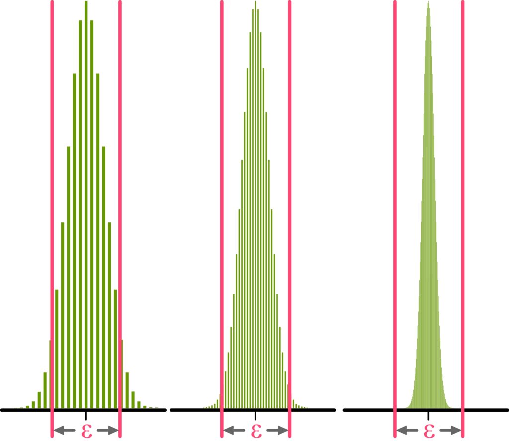
In the figure, the situation for the 40-fold, 100-fold, and 500-fold coin toss is shown.
Each sequence of heads and/or tails of length \(40\) is an outcome of the 40-fold coin toss. In the 100-fold coin toss, we get as outcomes sequences of heads and/or tails of length \(100\), and in the 500-fold coin toss, the outcomes are sequences of length \(500\).
To define what „close“ means, we simply place an interval of arbitrary length \(\epsilon\) around the probability of heads (namely \(0.5\)) and say: If the relative frequency of heads of an outcome (of the 40-fold, 100-fold, or 500-fold coin toss) lies within this interval, this means that the relative frequency of heads is close to the probability of heads (namely \(0.5\)).
As we can see, the proportion of outcomes lying within the interval becomes larger and larger as we repeat the experiment more often. The weak law of large numbers now states that this proportion (of the total outcomes) even tends to \(1\) (and the proportion of all other outcomes tends to \(0\)) if we repeat the coin toss an unlimited number of times.
Therefore, the probability that the relative frequency of heads is close to the probability of heads also becomes larger and larger. The weak law of large numbers states that this probability even tends to \(1\) if the coin toss is repeated an unlimited number of times.
It may seem somewhat curious that we chose \(\epsilon\) arbitrarily. The crucial point of the weak law of large numbers, however (and this is what makes the law so strong), is that it holds for all \(\epsilon\) – including very small ones.
In the following PDF, the weak law of large numbers is explained as simply as possible — but not simpler! It is presented in a mathematically correct way, but applied only to the simplest possible case, the coin toss. In addition, it shows how one can visualize this law and what kinds of misinterpretations exist.
Strong Law of Large Numbers
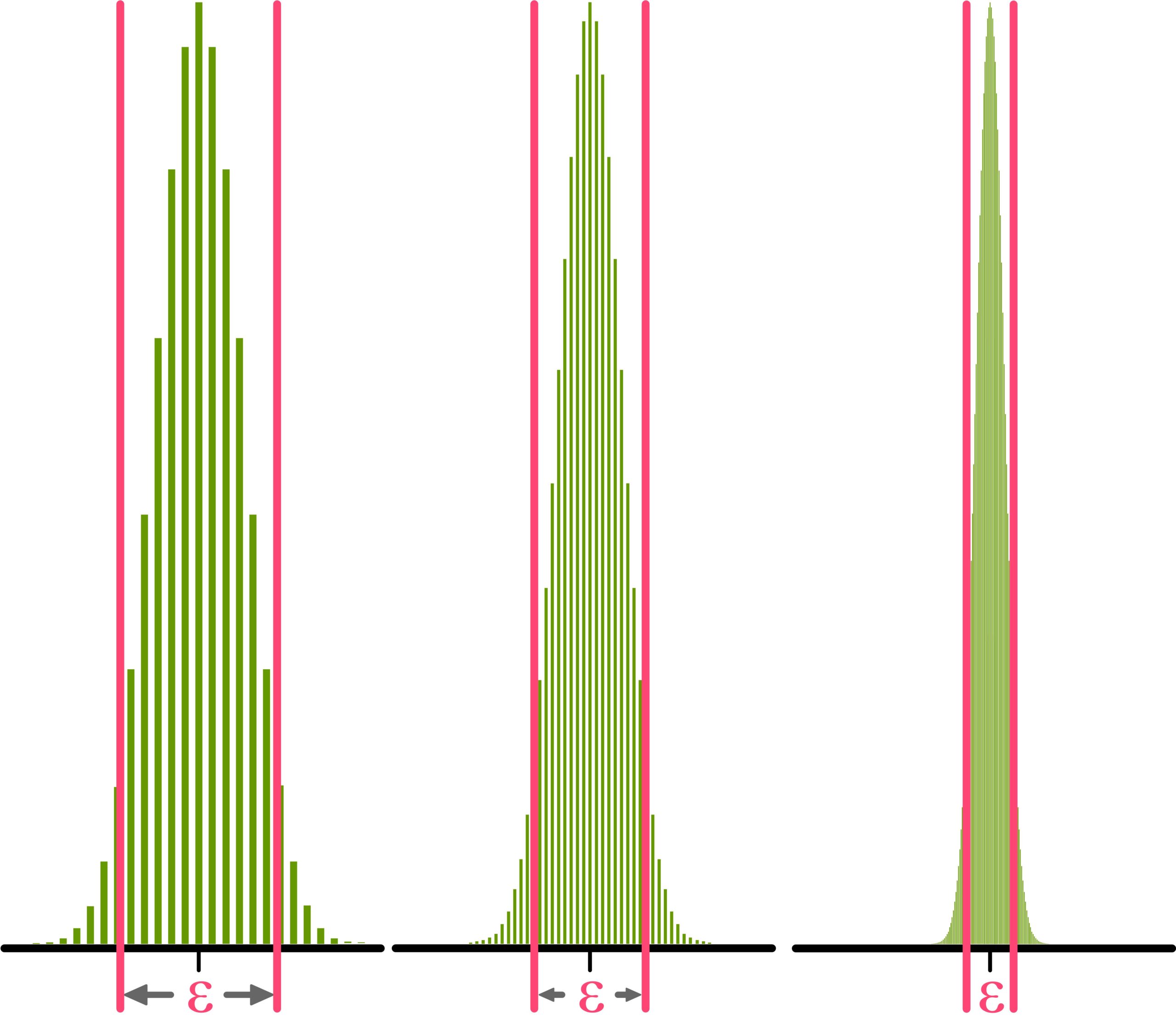
To understand the strong law of large numbers, we want to adopt the situation from the consideration of the weak law of large numbers. One of the major differences between the strong and the weak law of large numbers is that the strong law says something about what happens when we perform the coin toss infinitely many times. Let us look at the situation more closely:
If we toss a coin infinitely many times, the outcomes are infinitely long sequences of heads and tails, such as
(Heads, Heads, Tails, Heads, Tails, Tails, Tails, Heads, … )
Among these infinite sequences, there are some whose relative frequency of heads (in a certain mathematical sense) is equal to \(0.5\). These shall be called „\(0.5\)-sequences.“
And there are infinite sequences for which this is not the case. These shall be called „other sequences.“
The strong law of large numbers now states (in the simple framework we have set here): There are not only far more \(0.5\)-sequences than there are other sequences, but there are even (in a certain mathematical sense) infinitely more \(0.5\)-sequences than other sequences.
To illustrate this law and to better understand the logic behind it, we can again (as we did with the weak law of large numbers) look at the sequences of the 40-fold, 100-fold, and 500-fold coin toss in a figure. As with the weak law, for the 40-fold coin toss, we again placed an interval of arbitrary length \(\epsilon\) around \(0.5\). Unlike before, however, the interval length \(\epsilon\) now becomes smaller as the number of trials increases.
The strong law of large numbers now states that the proportion of outcomes within the \(\epsilon\)-interval becomes larger and larger as the number of trials increases, even if \(\epsilon\) becomes smaller and smaller. More precisely: If the coin toss is performed infinitely many times, the proportion of outcomes within the \(\epsilon\)-interval tends to \(1\) even as \(\epsilon\) tends to \(0\) (and the proportion of outcomes outside the \(\epsilon\)-interval tends to \(0\)). For the infinite \(0.5\)-sequences, this then means (in a certain mathematical sense) that their proportion (of all sequences) is infinitely larger than the proportion of the other sequences.
The following PDF explains the strong law of large numbers. It does not present a simplified or informal version of the law, but the actual mathematical law — though it is explained only for the simplest possible case, the coin toss. All formal necessities, such as the means of centered random variables, are explained in the text. Everything that is not absolutely essential is omitted. In addition, the usual misinterpretations are discussed and corrected.
Stochastic Independence – Visual Explanation
The stochastic independence of two events is defined by a formula that, from a visual or graphical standpoint, does not reveal much. However, to understand it on an intuitive level, we can turn to a visual interpretation. There, we will see that stochastic independence concerns the relationship between two sets. When this relationship is, in a certain sense, harmonious, the events are stochastically independent.
More precisely, the events A and B are stochastically independent exactly when the proportion of A within the sample space is equal to the proportion of the intersection of A and B within B.
This perspective is especially important because schools often teach that stochastic independence requires two random experiments. According to the formula, however, that is not correct, since the events A and B are subsets of the sample space of one and the same random experiment.
There is also a common misconception that events A and B have “nothing to do with each other” or “do not influence each other” when they are stochastically independent. But in principle, events of a random experiment are simply subsets of the sample space; they just exist — they do not, and cannot, actively influence one another.
Conditional Probability – Simple Explanation
In this video, we first look at the formula that defines conditional probability. However, the formula itself is rather bare, so we will also look at a diagram that allows us to visualize conditional probability in a much clearer way. This will lead us to a formulation of conditional probability in “ordinary” words.
For example: Let A and B be events of a random experiment. The probability of A given B — written as P(A|B) — is the portion of A within B.
Alternatively, we can say: The probability of A given B is the proportion of the probability of A relative to the probability of B.
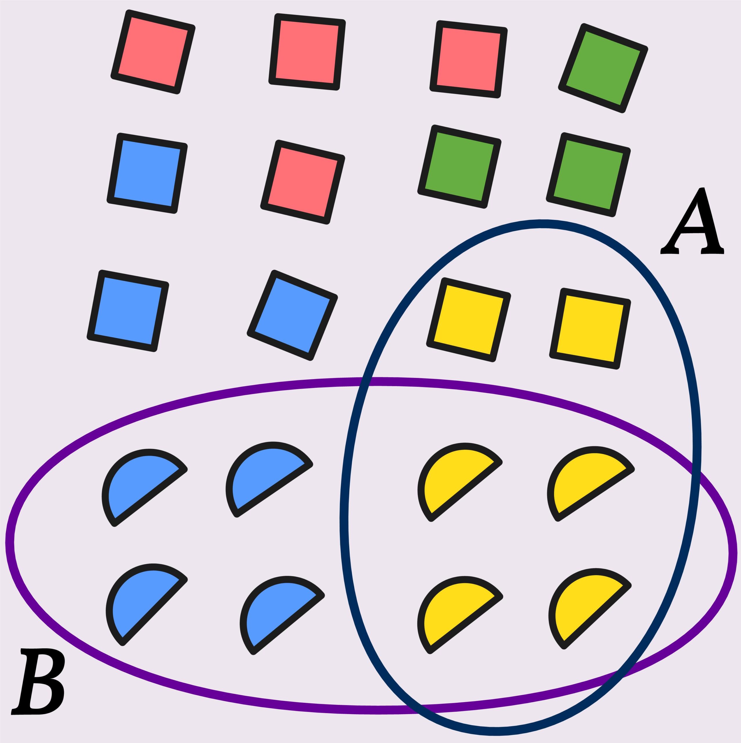
In the situation shown on the right, we are dealing with the random experiment: a single random draw of one figure.
Set A contains all yellow figures, and set B contains all half-circles.
The probability of A given B — that is, P(A|B) — is (in this case) the proportion of yellow half-circles among all half-circles, that is, the proportion of A within B.We have:\[ P(A|B)= \frac{1}{2} \]
There are many persistent misconceptions about the concept of conditional probability. For example, it is often claimed that two random experiments (or at least two actions within one random experiment) are required in order to define conditional probabilities. According to this idea, “the probability of A given B” is said to be the probability that A occurs when B has already occurred — or, in other words, the probability that A occurs on the second trial if it is already known that B occurred on the first trial.
This incorrect notion makes it impossible to solve certain problems involving conditional probability. For example: A container holds two black and two white balls. Two draws are made without replacement. The question is: What is the probability that a black ball is drawn first, given that a white ball is drawn second?
If one holds the belief that only the first draw can serve as a condition for the second draw, one will likely conclude that the problem is formulated incorrectly. However, if the sample space is written out with all possible pairs of draws and the problem is treated as shown in the video, this apparent contradiction will (certainly) be resolved.
Miscellaneous
Project: Infinity
Infinity is a fascinating topic in mathematics.
Below is a list of ideas that could be used for a math project on this theme.
These are questions that usually do not appear immediately in AI search results and that (mostly) have their roots in school mathematics.
They can, however, be explored with AI, since there are no standard answers to them.
How far can one count?
Is there a largest number?
What could very large numbers count?
All the grains of sand on Earth?
All possible ways to arrange the books in a library?
All possible books that could be written?
Is there a total number of all possible thoughts one could think?
Can one write down a number so large that it exceeds everything one could reasonably count?
And to what extent does such a number exist if it counts nothing at all?
Suppose God wanted to create a new living being and place it on Earth.
Then one could also take a photograph of that being.
However, with ordinary technical means, there are only finitely many possible photos (since a screen has finitely many pixels, and each pixel can take only finitely many colors and brightness levels).
Does that mean that God has only finitely many possibilities to create a new being?

If the number \(1\) represents a certain step length along a circle, one can take infinitely many steps without ever moving away from the circle’s center.
In a sense, numbers would then never become infinitely large.
Is a circle infinite? Is the surface of a sphere infinite?
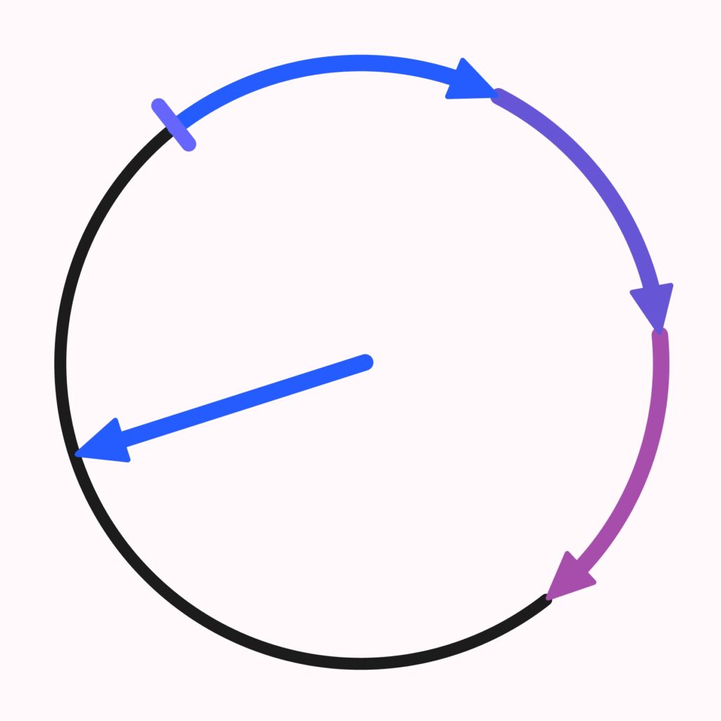
You can choose a starting point on a circle and lay the circle’s radius, beginning at that point, along the circle’s circumference. Then you can place the radius again, and again, and so on.
Will one of the endpoints of these radii ever coincide with the starting point?
Suggestion: If you add \(1\) to a very large number, it becomes larger, but—compared to its size—not much larger.
Ultimately, numbers grow by repeatedly adding \(1\), but they never become infinitely large, because what is added becomes relatively smaller and smaller.
In mathematics, we study numbers that have infinitely many decimal places.
But how can such numbers exist if we cannot write them down as decimals?
Is \(0.999 \dots \) actually equal to \(1\)?
Why does that sound strange?
If \(0.999 \dots \) were not equal to \(1\), how large would the distance between \(0.999 \dots \) and \(1\) have to be?
Can one divide infinity by \(2\) ? Or by infinity?
Are there half as many even numbers \((2, 4, 6, 8, …)\) as natural numbers \((1, 2, 3, 4, …)\)?
One can assign to every natural number n an even number, for example \(f(n)=2n\).
Since every natural number corresponds to exactly one even number, and every even number corresponds to exactly one natural number, are there just as many even numbers as natural numbers?
Can one, using ordinary craft materials (paper, crayons, scissors, glue, cardboard tubes, small parts, liquids, etc.), start a process that adds something (at least theoretically) endlessly often to a whole—without the whole becoming infinitely large?
Can one, with ordinary craft materials, divide something again and again without it becoming infinitely small?
Maybe if one divides by fractions such as \(\frac{99}{100}\), \(\frac{999}{1000}\), \(\frac{9999}{10000}\), and so on?
Why does the sum \(\frac{1}{2} + \frac{1}{3} + \frac{1}{4} + \dots\) grow without bound, even though its terms become smaller and smaller (approaching \(0\)), while the sum \(\frac{1}{2^2} + \frac{1}{3^2} + \frac{1}{4^2} + \dots\) does not?
If m is a positive number, the values of the function \(f(x)=mx+b\) (for any \(b\)) go to infinity as x goes to infinity.
The same is true for \(g(x)=mx^2+b\).
But \(g(x)\) seems to approach infinity faster than \(f(x)\).
What could that mean?
How do other functions behave—power functions, exponential functions, root functions, logarithmic functions?
Could there be a slowest-growing function that still goes to infinity?
The sequence of numbers \(\frac{1}{2}, \frac{1}{3}, \frac{1}{4}, \frac{1}{5}, \dots\) tends to \(0\), even though none of its terms is equal to \(0\).
Does that make sense to you?
Using Cantor’s diagonal argument, one can show that there are more real numbers than can be counted.
That is why we say that the real numbers are uncountable.
How can that be imagined?
With cardinal numbers, one can describe the sizes (cardinalities) of sets.
Moreover, the set of all subsets of a set (the power set) always has a greater cardinality than the set itself.
Therefore, the power set of the real numbers is a beyond-uncountable set.
How can that be imagined?
What kinds of numbers arise if we continue the process of forming power sets indefinitely?
Introductory Teaching Video
Here is an introductory teaching video on the topic of volumes. It shows how much liquid can be “poured into” a standard pizza plate – with a result that is surprising for many people.
This teaching entry can be easily connected to the question: Why do we need mathematics? In this case, the short answer is: besides the fact that understanding mathematics is fun for everyone, the example of the plate shows that humans are very bad at estimating and comparing volumes. With the help of mathematics, however, we can calculate volumes precisely and don’t have to – as in the shown case – experiment with milk.
Examples where experimenting can be problematic:
1. When planning a swimming pool, the required amount of water must be calculated during the planning phase. To determine the heating power needed to warm the water (as is common in public pools), you must know the volume of water in the pool.
2. A water-filled aquarium is heavier than most people expect. For the sake of the fish inside, one should not simply experiment to see if the aquarium is safe on a lightweight shelf.
3. Topsoil is often sold in 20-liter bags. When planning a school garden, calculating the required volume of topsoil helps determine the financial effort.
Examples where humans usually misjudge:
1. Pour 1000 small cubes (1 cm edge) into a pile and place a cube (e.g., made of paper and foldable) with a 10 cm edge next to it. Ask: how many of the small cubes fit into the large cube? (Experience shows answers range between 100 and 300.) Correct answer: all of them.
2. What is the radius of a sphere whose volume equals that of a human? For students of the corresponding age, r ≈ 25 cm is a reasonable estimate.
3. Questions about double volumes: What is the edge length of a cube whose volume is twice that of a given cube with edge length k? (Answer: approximately 1.26·k.) The same applies to a sphere with double volume and the height of a sand pile with double volume.
The Standard Model of School Mathematics
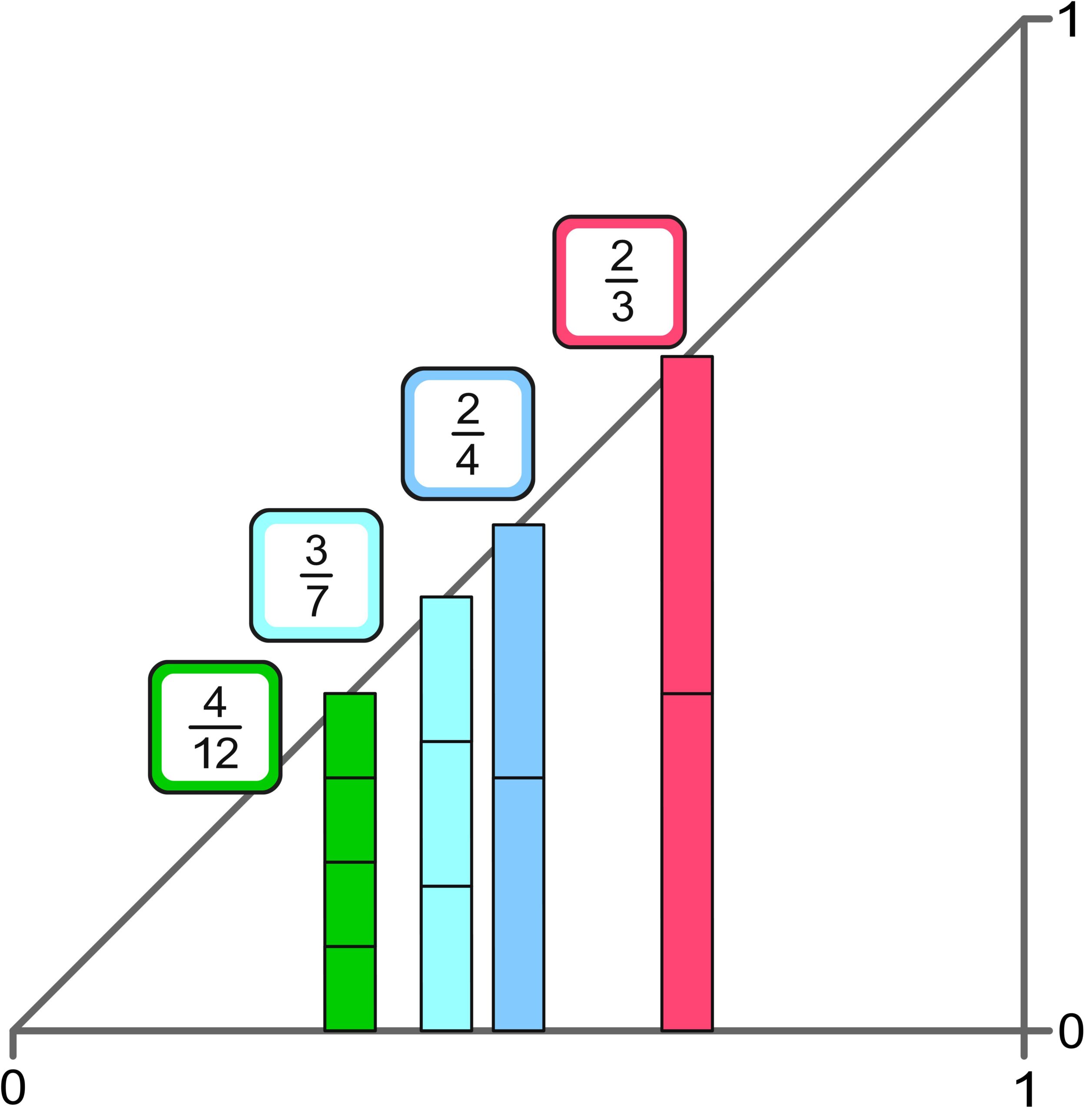
We can think of numbers as line segments on the number line. But we can also arrange them vertically, which allows us to see many relationships that are not visible with “horizontal” numbers. For example, the multiplication of fractions or exponentiation with rational exponents can be very clearly understood using this model.
Sorry, no English version abailable at the moment.
Position Vector – Definition
A position vector is not a vector that is located at a certain place; rather, a position vector is a vector that is defined by a location. Locations are points in the coordinate system. Once a location is fixed, there is exactly one arrow that leads from the origin of the coordinate system to that point. This arrow represents exactly one vector — namely, the position vector defined by that point. In the video, we will also look at this idea graphically.
This video is especially suitable for people who value a mathematically precise yet visually intuitive definition of the position vector. For that reason, it focuses specifically on how one can understand that, although the position vector is defined by a location and there is only one arrow that leads from the origin to that point, this vector itself is nevertheless not bound to that location.
Anyone who has completed the marathon of searching the internet for an exact and contradiction-free definition of the position vector will be greatly relieved by the end of the video.
Surface Area of a Sphere – Cosmetics and Nanoparticles
Let a sphere be given. If we divide the volume of this sphere into several smaller spheres, we find that the sum of the surface areas of the smaller spheres is greater than the surface area of the original large sphere. The smaller the spheres are, the larger the total surface area becomes.
In everyday life, extremely small “spheres” sometimes occur. For example, C₆₀ fullerenes are incorporated into certain cosmetic products. C₆₀ fullerenes are molecules that resemble small soccer balls. Among other reasons, because these molecules have a very large surface area per unit volume, they are highly chemically reactive. This also means that—if they have undesirable side effects such as toxicity—these side effects can be very strong.
In this video, we will examine mathematically how the total surface area increases as the size of the spheres decreases. By the way, this same issue can also be found in many areas of everyday life—for instance, in fine particulate matter (fine dust) that we inhale.
Mathematical Induction
Mathematical induction is a proof method that is (usually) used to show that a statement holds true for every natural number. It consists of two steps:
- You show that the statement is true for a first number—usually for 1.
- You show that if the statement is true for a certain number, then it is also true for the following number. From this, you conclude that the statement holds true for all natural numbers.
In the video, you will see how to understand this method in an intuitive, visual way, because—in a sense—we apply this method, for example, whenever we walk somewhere. After that, you can see several examples in which statements are proven using the method of mathematical induction.
Help! My Child Can’t Do Math!
Even when it feels as if nothing is working anymore, there are still ways to deal with the situation—either well or poorly.
Unfortunately, I often see cases where, for example, a grade of F in math is turned into a much bigger problem, to the point where the child is even declared ill and must then be treated by a dyscalculia therapist.
A respectful attitude and an optimistic mindset, however, can allow the situation to remain what it actually is: a single number written on a test paper.